Methods: Quadratic programming und SOCP
Definition

Quadratic programming (QP), quadratically constrained quadratic programming (QCQP), and second order cone programming (SOCP) are generalizations of linear programming (LP). They encompass many practical problems, including generalizations of least squares.
The linear objective function and linear constraints of LP are extended to quadratic objective functions and quadratic constraints. Quadratic programs have the form:
\[
\begin{align*}
\text{(QP)} \quad & \min_x \quad \frac{1}{2} x^T P_0 x + \langle c_0, x \rangle \\
&~ \text{s.t.} \quad Ax = b \\
& \quad Gx \ge h
\end{align*}
\]
\[
\begin{align*}
\text{(QCQP)}\quad & \min_x \quad \frac{1}{2} x^T P_0 x + \langle c_0, x \rangle \\
& ~\text{s.t.} \quad Ax = b \\
& \quad \frac{1}{2} x^T P_k x + \langle p_k, x \rangle \le h_k \quad k=1, …, m_2
\end{align*}
\]
where \(x, c_0, b, h\) are vectors and \(P_0, P_1, …, P_{m_2}, A, G\) are matrices. QP directly extends LP by incorporating the quadratic term \((1/2) x^T P_0 x\) in the objective function, and QCQP extends QP by including quadratic terms \((1/2) x^T P_k x\) in the constraints, involving circle and ellipsoid equations. SOCP investigates an even more general optimization problem:
\[
\begin{align*}
\min_x & \quad \langle c, x \rangle \\
\text{s.t.} & \quad Ax = b \\
& \quad \|G_k x + h_k\|_2 \le \langle f_k, x \rangle + d_k \quad k=1, …, m_2
\end{align*}
\]
in the optimization variable \(x\), where \(x, c, b, f_1, …, f_{m_2}, h_1, …, h_{m_2}\) are vectors, \(A, G_1, …, G_{m_2}\) are matrices, and \(d_1, …, d_{m_2}\) are scalars.
Example
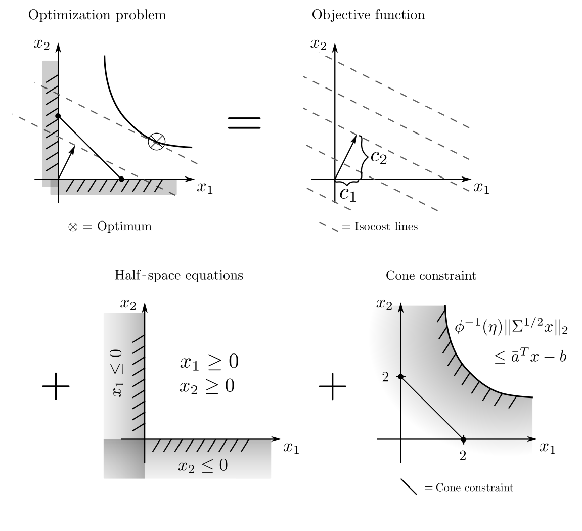
SOCP allows for the solution of linear programs where the conditions are stochastic in nature. Suppose two products are to be manufactured in quantities \(x_1, x_2\) such that the demand \(b\) is met while minimizing production costs \(c_1x_1 + c_2x_2\). Now, consider that the production process is subject to uncertainties, so that only parts \(a_1x_1, a_2x_2\) of the manufacturing output are usable. If \([a_1, a_2]\) are random, it makes sense to require the fulfillment of the demand not absolutely but with high probability \(\eta\). If \(a=[a_1, a_2]\) is normally distributed with mean \(\bar{a}=[\bar{a}_1, \bar{a}_2]\) and covariance matrix \(\Sigma\), then
\[
\begin{align}
P(a^Tx \ge b)\ge \eta & \Leftrightarrow \phi^{-1}(\eta) \|\Sigma^{1/2} x \|_2 \le \bar{a}^Tx — b
\end{align}
\]
where \(P(\cdot)\) stands for the probability of the enclosed expression and \(\phi^{-1}\) is the inverse of the cumulative normal distribution function. The corresponding SOCP
\[
\begin{align}
\min_x ~~~& c_1x_1 + c_2x_2 \\
\text{s.t.} & x_1 \ge 0 ~~~ x_2 \ge 0 \\
& \phi^{-1}(\eta)\|\Sigma^{1/2}x\|_2 \le \bar{a}^Tx‑b
\end{align}
\]
formulates a cost minimization while ensuring a probability of demand coverage of \(\eta\)% [1, p.158]. The subsequent figure illustrates this for the case \(\bar{a}=[0.7, 0.7], \Sigma=0.1 I\), and \(\eta=90\%\); the other parameters are as in the example for LP.

Geometrical aspects
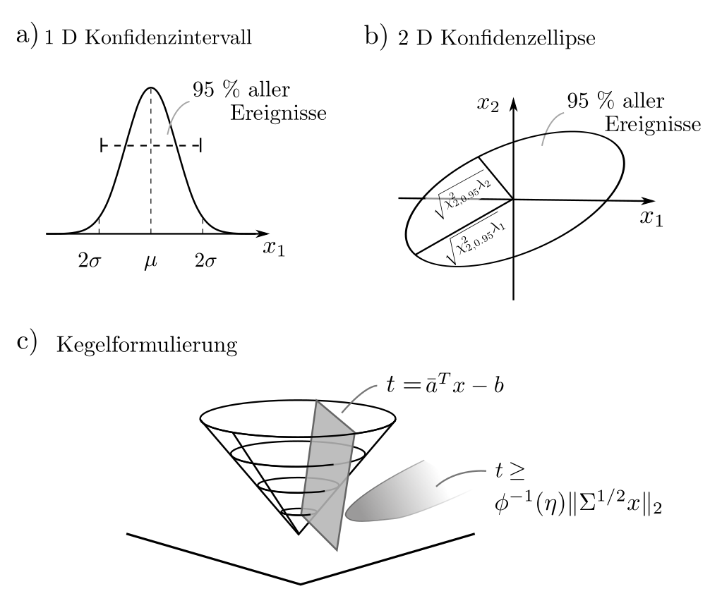
The cone condition \( \|\Sigma^{1/2} x\|_2 \le [\phi^{-1}(\eta)]^{-1}(\bar{a}^Tx‑b)\) is a multivariate generalization of the classical confidence intervals. While these are actual intervals in the one-dimensional case, in the two-dimensional case they take on ellipsoid-like shapes. The term \(\| \Sigma^{1/2} x\|_2\) is the standard deviation of the random linear combination \(a^Tx\) and thus a measure of the dispersion around the expected value \(\bar{a}^Tx\).
Both measures are needed to estimate the probability that the share \(a^Tx\) of defect-free products falls short of the required demand due to random fluctuations. Since \(\|\Sigma^{1/2} x\|_2\) and \(a^Tx\) appear on both sides of the equation, it can only be formulated as an SOCP, not as a QCQP.

Applications
All examples of applications of LP are also examples of applications of SOCP. In particular, problems that involve vector lengths and ellipsoids can be formulated, which include stochastic generalizations of LP and the minimization of physically motivated quadratic energies. Specifically, these are portfolio optimizations, robust LP, LP with stochastic constraints, optimal linear-quadratic control of kinematic systems, physical simulation, parameter estimation in Gaussian models, robust Least-Squares, Kalman filtering, isotonic regression, antenna design, robot trajectory optimization, and image processing. Details can be found here.
The examples seem less practically relevant and intuitively understandable than with LP. However, this is because QP, QCQP, and SOCP extend the classical LP to include the presence of uncertainty and provide new possibilities for other established techniques such as Least-Squares.
Solution procedure
Since the feasible sets are curved, searching for the optimum by enumerating and evaluating all vertices is not practical. Solution approaches with a particular emphasis on speed are often gradient-based, as the gradients of quadratic and linear terms are simple to calculate. These include methods such as conjugate gradients, augmented Lagrangian, and projected gradients [2, pp. 73, 116, 173]. Due to their universal applicability and increasing numerical performance, interior-point methods are also increasingly used, which substitute constraints with additional penalty terms.
Practical aspects
SOCPs with many tens of thousands of variables can reliably be solved today. Solution algorithms are available in the form of open-source software, such as the Splitting Conic Solver [3]. Due to the closeness of QP to finite element methods, there is also software specifically for applications in structural engineering and mechanical engineering [4]. Given the frequent occurrence of quadratic energy terms in physics, mechanics, and statistics, QP is a natural tool in these disciplines. The correct form of QPs and QCQPs may be directly discernible from a problem formulation; SOCPs are typically harder to interpret. If not all embeddings were obvious in LP, this is even more the case here.
Code & Sources
Example code: Methods_socp.py in our tutorialfolder
[1] Boyd, S., & Vandenberghe, L. (2004). Convex Optimization. Cambridge: Cambridge University Press.
[2] Dostál, Zdenek. (2009) Optimal Quadratic Programming Algorithms: With Applications to Variational Inequalities. Berlin Heidelberg: Springer Science & Business Media.
[3] O’donoghue, B., Chu, E., Parikh, N., & Boyd, S. (2016). Conic Optimization via Operator Splitting and Homogeneous Self-Dual Embedding. Journal of Optimization Theory and Applications, 169(3), 1042–1068.
[4] Szabo, B. A., & Tsai C. (1973). The quadratic programming approach to the finite element method. International Journal for Numerical Methods in Engineering, 5(3), 375–381.
