Methods: Linear programming
Definition

Under linear programming (LP), all optimization problems are grouped whose objective function and constraints are of a linear nature. It is the simplest class of optimization problems that require numerical solution approaches. They can all be written in the form:
$$ \begin{align} \min_x ~~~& \langle c,x\rangle \\ \text{s.t.} ~~~&Ax=b \\ ~~~& Gx\ge h \end{align}$$
in the optimization variable \(x\), where \(x, c, b, h\) are vectors and \(A, G\) are matrices. The above problem in detailed notation is as follows.
- Find the variables \(x_1, …, x_n\) such that \(\langle c,x\rangle = c_1x_1 + \dots + c_nx_n\) is minimized.
- The following conditions needs to be satistified:
- \(a_{k1} x_1 + , …, + a_{kn}x_n =b_k ~~~~k=1, …, m_1\)
- \(g_{k1} x_1 + , …, + g_{kn}x_n \ge h_k ~~~~k=1, …, m_2\)
The problem consists of a sum \(\langle c,x\rangle\) to be minimized, \(m_1\) equalities, and \(m_2\) inequalities. All terms are linear in the optimization variable \(x\), hence the name “linear programming”.
Example
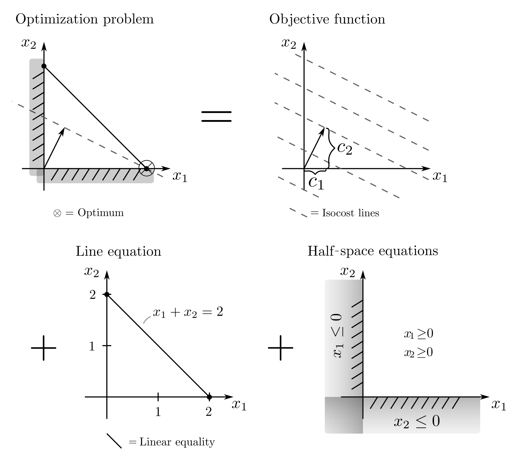
LP involves archetypal economic production problems such as production planning [1, pp. 14–16]. For instance, if \(x_1, x_2\) are the quantities of two products with production costs \(c_1, c_2\), then the optimization problem
$$ \begin{align} \min_x ~~~& c_1 x_1 + c_2 x_2 \\ \text{s.t.} ~~~&x_1 + x_2 =2 \\ ~~~& x_1 \ge 0 ~~~ x_2 \ge 0 \end{align}$$
can be interpreted as an instruction to minimize production costs while covering a total demand of 2. Negative production quantities are not allowed. Extensions of this example to multiple products, minimum demands, and resource consumption constraints are easily feasible.

Geometrical aspects
The above example has a clear geometric interpretation as determining a two-dimensional point \(x = [x_1, x_2]\) that is constrained in its position by some lines.
The optimum is reached at the vertex of the feasible set through which the line of minimal cost equivalence runs. In high-dimensional problems, two-dimensional vectors become n‑dimensional vectors, line equations become hyperplane equations, and the inequalities define half-spaces. The fundamental geometric properties and interpretations remain the same.
Applications
The applications of linear programming extend far beyond production planning. They include problems from logistics, transportation and routing planning, machine scheduling, inventory control, diet design, material flow, factory layout, stochastic inequalities, image quality optimization, data compression, robust approximation, game theory, and logic. Depending on the application, \(\langle c,x\rangle\) represents monetary costs, negative profit, durations, maximum deviations, probabilities, or auxiliary quantities that are difficult to interpret. More details on these applications can be found here. The representations of these problems as LP are often not obvious.
Solution procedure
Linear programs are historically the first high-dimensional optimization problems relevant to real-world applications that could be reliably solved. In the context of planning problems for the US Air Force after World War II, Dantzig developed the so-called Simplex Method, whose further development and use for resource allocation problems helped Koopmans and Kantorovic win a Nobel Prize in Economics [2, p. 10].
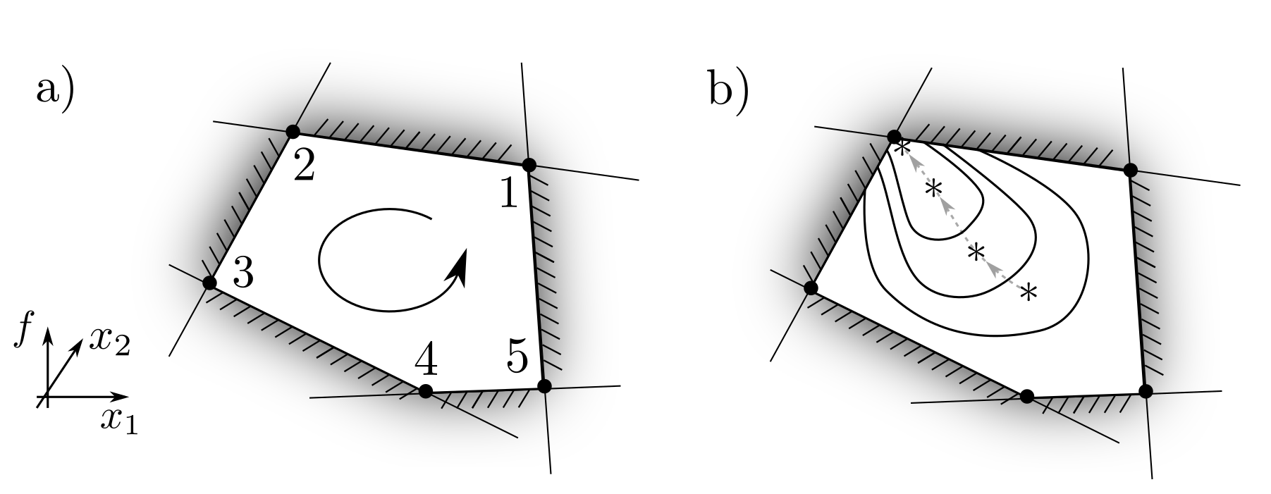
As already noted in Figure 1 and generally provable, the optimal point \(x\) of an LP is located at one of the vertices of the feasible set defined by the intersections of hyperplanes. Enumerating and sequentially testing each vertex leads to the reliable identification of the optimum [3, p. 72]. Since the number of vertices can grow disproportionately with the number of dimensions, this complete enumeration is often costly, and better methods now exist; the interior-point methods. These methods involve replacing the inequalities with barrier functions, whose weight is incrementally reduced, thereby generating a sequence of points—the central path—that converges to the optimum.

Practical aspects
LPs with hundreds of thousands of optimization variables are now well solvable on commercial home computers. Open source algorithms such as those implemented in the GNU Linear Programming Kit (GLPK) or Google’s GLOP solver are available for this purpose. The fact that even Excel is now capable of solving LPs can be seen as further evidence that LP has reached technical maturity. The main challenge lies in the formulation of the optimization problem itself.
Sources
[1] Hu, T. C., & Kahng, Andrew B. (2016). Linear and Integer Programming Made Easy. Berlin, Heidelberg: Springer.
[2] Vanderbei, Robert J. (2013). Linear Programming: Foundations and Extensions. USA: Springer US.
[3] Gass, Saul I. (2003). Linear Programming: Methods and Applications. New York: Courier Corporation.
