Dynamic programming - Atlas optimization

Methods: Dynamic programming

Definition

Dynamic programming (DP) addresses optimization problems where the optimization variables represent sequences of decisions. This sequentiality is used to establish recursive relationships for the value of specific states and actions of the system.

This recursion breaks down the overall problem into a sequence of interdependent subproblems that can be solved efficiently. Therefore, DP is both a solution approach and a class of problems. For clarity, we interpret DP more narrowly than necessary as the optimization problem

$$ \begin{align} \min_{\pi} ~~~& f(\pi) \\f(\pi)
~~~&= \sum_{k=1}^{end} E\left[ r(s_k, s_{k+1}, \pi(s_k))\right] \end{align}$$

where the optimization variable is $\pi$ [1, p. 23]. The peculiarity lies in the interpretation of $f(\pi)$ as the expected reward $E[r]$ in response to actions $\pi(s_k)$ dependent on system states $s_k$. The goal is to find a policy $\pi$ that maps system states to control inputs that optimally steer the system on average. The quality of a solution is measured by the cumulative amount of reward $r$ collected.

Example

Imagine, for example, a continuous inventory planning scenario where cost-minimizing decisions need to be made based on current stock levels and sales opportunities that become known over time. Inventory shortages lead to loss of profit, while excess inventory incurs storage costs.

In the above example, it is clear that a constant reorder rate is suboptimal and decisions on order quantities depend on current inventory levels, demand, and expected changes in both parameters. Formulating the entire matter as a single function $f$ seems difficult, and indeed, the situation is best represented as a Markov Decision Process (MDP).

MDP

A Markov Decision Process (MDP) is a controllable stochastic process. It consists of a 4‑tuple $\{S, A, P, R\}$ which defines the dynamics of the process.

$S$ is a set of states $s$.
$A$ is a set of actions $a$.
$P(s’| s, a)$are the transition probabilities from $s$ to $s’$ when action $a$ is chosen.
$R(s’| s, a)$ )\) is the reward for transitioning from $s$ to $s’$ via action $a$.

Thus, it involves a set of states $s$ of a system that evolves under the influence of actions $a$. The subsequent state $s’$ depends on $s, a$, and randomness, while the reward depends on $s’, s, a$. The goal is to maximize cumulative rewards. To achieve this, the optimal action for each state must be determined. The function $\pi: s \mapsto a$ is also called a policy.

Application example

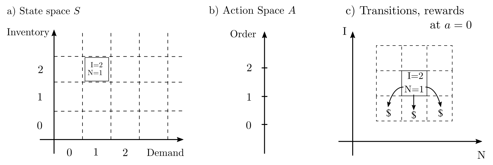
In the context of the inventory planning example, $S=\mathbb{R}^2$ because the state is characterized by two numbers: inventory and demand. Furthermore, $A=\mathbb{R}$, $R(s’, s, a)$ represents the balance between sales profit and storage costs, and the transition probabilities reflect $\text{Inventory}’=\text{Inventory}-\text{Demand}+a$ along with a random shift in demand.

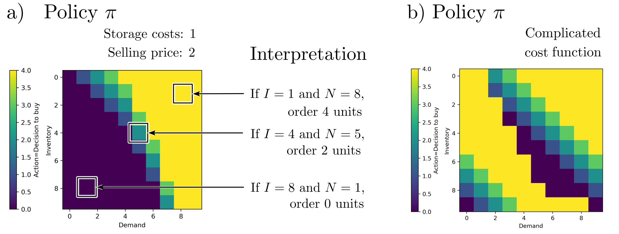
The result of DP is the policy $\pi:s\mapsto a$, which maps states $s=(B, N)$ to product reorder actions $a$. In this case, it is a scalar field with an input dimension of 2 (the states) and an output dimension of 1 (the actions).

A policy generated in this way can now be used in practice to determine the most promising actions for each configuration of inventory and demand. Thus, a policy is more than just a rigid plan—it is an adaptive set of measures.

Applications

DP, especially in the context of MDPs, is primarily used for optimal system control. Even in its simplest form, the formalism is capable of handling nonlinear rewards, discrete control signals, and complex transition probabilities, and converting them into optimal policies. The unique aspect of policies is that they are flexible action plans that propose sequences of actions for all possible states, thus allowing them to respond appropriately and effortlessly to unforeseen events.

Plans using other methods, such as production planning with LP, provide only a single sequence of optimal decisions starting from an initial state and offer less flexibility and adaptivity. Therefore, DP is often used in operational areas where decisions need to be made quickly and data for probabilistic modeling is available. This is the case, for example, with dynamic control of traffic lights, ambulance dispatches, communication networks, supply chains, and water management processes, and extends to predictive scheduling in medicine, occupancy planning in call centers, and the development of fishing policies. Details can be found here.

Solution

In simple cases, characterized by a finite number of states and a manageable number of discrete actions, MDPs can be solved through iterative methods. To maximize the term

$$E_{\pi}\left[ \sum_{k=1}^{\text{end}} r(s_{k+1}, s_k, \pi(s_k))\right]$$

representing the expected total reward, a function $V_{\pi}(s)$ is typically introduced. This so-called value function measures the expected total reward when starting from state $s$ and following the policy $\pi$. For arbitrary states $s$ and $s’$, $V_{\pi}(s)$ and $V_{\pi}(s’)$ are functionally related. Alternating iteration to determine $V_{\pi}$ and to optimize $\pi$ is called value iteration [1, p. 37] and leads to the optimal policy $\pi^*$.

Figure 4: The iteration progressively refines the estimates for the value function and the policy, deriving the value function $V_{\pi^*}$ of the optimal policy $\pi^*$ (a). In (b) and ©, the functional relationship between $V_{\pi}(s)$ and $V_{\pi}(s’)$ is symbolized. Following policy $\pi$ in state $s$ leads to states $s_1’, s_2’, …$, and corresponding rewards $r_1, r_2, …$ with probabilities $p_1, p_2, …$. This implies functional relationships on the value function. Illustrations are based on [3, p. 87].

Dynamic Programming (DP) for Markov Decision Processes (MDPs) in infinite-dimensional spaces is also possible and necessary when more than a finite number of potential states or actions must be considered. This involves solving sequences of linear programs [1, p. 377]. If states are only partially observable or if the model of state transitions is entirely unknown, formulations as Partially Observable Markov Decision Processes (POMDPs) or as Reinforcement learning problems are possible.

Practical aspects

Dynamic Programming (DP) and Markov Decision Processes (MDPs) are effectively solvable with open-source algorithms such as those provided in the pymdp Toolbox for Python. However, these algorithms are less extensively tested and maintained compared to those available for LP, QP, etc. Solving optimal control problems via DP and MDP has a more experimental character. Nonetheless, it is often the only approach that adequately addresses the complexity of real-world problems [2]. Both modeling the problem by formalizing state spaces and transition matrices, and the effective solution of MDPs are challenging.

Code & Sources

Example code: Methods_mdp.py in our tutorialfolder

[1] Feinberg, E. A., and Shwartz, A. (2012). Handbook of Markov Decision Processes: Methods and Applications. Berlin Heidelberg: Springer Science & Business Media.

[2] Boucherie, R. J., & Dijk, N. M. (2017). Markov Decision Processes in Practice. Heidelberg, New York, Dordrecht, London: Springer International Publishing.

[3] Sutton, R. S., & Barto, A. G. (2018). Reinforcement Learning: An Introduction. Cambridge: MIT Press.