Duality - Atlas optimization

Theory: Duality

Definition

For any given minimization problem, there exists a corresponding mirrored maximization problem known as the dual problem. This dual problem aims to find a lower bound for the minimum value of the original (primal) problem.

The solution of the dual problem provides insights into the impact of constraints on the location of the optimum. This allows for sensitivity analyses, which help answer questions related to system designs that contribute to the robustness of the optimum. Dual problems often resemble the underlying (primal) problem. For example, if

$\begin{align} P~~~~~~\min_x ~~~&f(x) \\ \text{s.t.} ~~~&A(x) =b \\ & G(x)\le h \end{align}$

is a general minimization problem, then the corresponding dual problem is

$\begin{align} D~~~~~~ \max_{\nu,\lambda} ~~~&\underbrace{\inf_x \left(f(x)+\nu^T(A(x)-b)+\lambda^T(G(x)-h)\right)}_{g(\nu,\lambda)} \\ \text{s.t.} ~~~&\lambda \ge 0 \end{align}$

where $\nu, \lambda$ are the vector-valued dual optimization variables, and $\inf_x$ is infimum over $x$ , robust against limit formation. More detailed information can be found in [1, pp. 215–230].

Relevance

For every feasible $x$ of the primal problem, the term $f(x)+\nu^T(A(x)-b)+\lambda^T(G(x)-h)$ is less than $f(x)$ , because for $\lambda \ge 0$ , it holds that $\nu^T(A(x)-b)=0$ and $\lambda^T(G(x)-h)\le 0$ . Consequently,

$g(\nu,\lambda) \le \min_{x\in D} f(x) ~~~D=\{x \in \mathbb{R}^n: A(x)=b \text{ und } G(x)\le h\}$

for all $\lambda \ge 0$ and $\nu \in \mathbb{R}^{m_1}$ . If $g(\nu,\lambda)$ is known, the minimum value of $P$ can be easily estimated. Maximizing over this lower bound leads to the dual problem $D$ , whose solution $d^*$ is the best derivable lower bound for the solution $p^*$ of the primal problem. The advantages of this formalism are threefold:

Sometimes $P$ is difficult, but $D$ is simple
Solutions $\lambda^*, \nu^*$ of $D$ provide insights into $P$
The duality gap $p^*-d^*\ge 0$ indicates whether $P$ and $D$ are correctly solved

Example

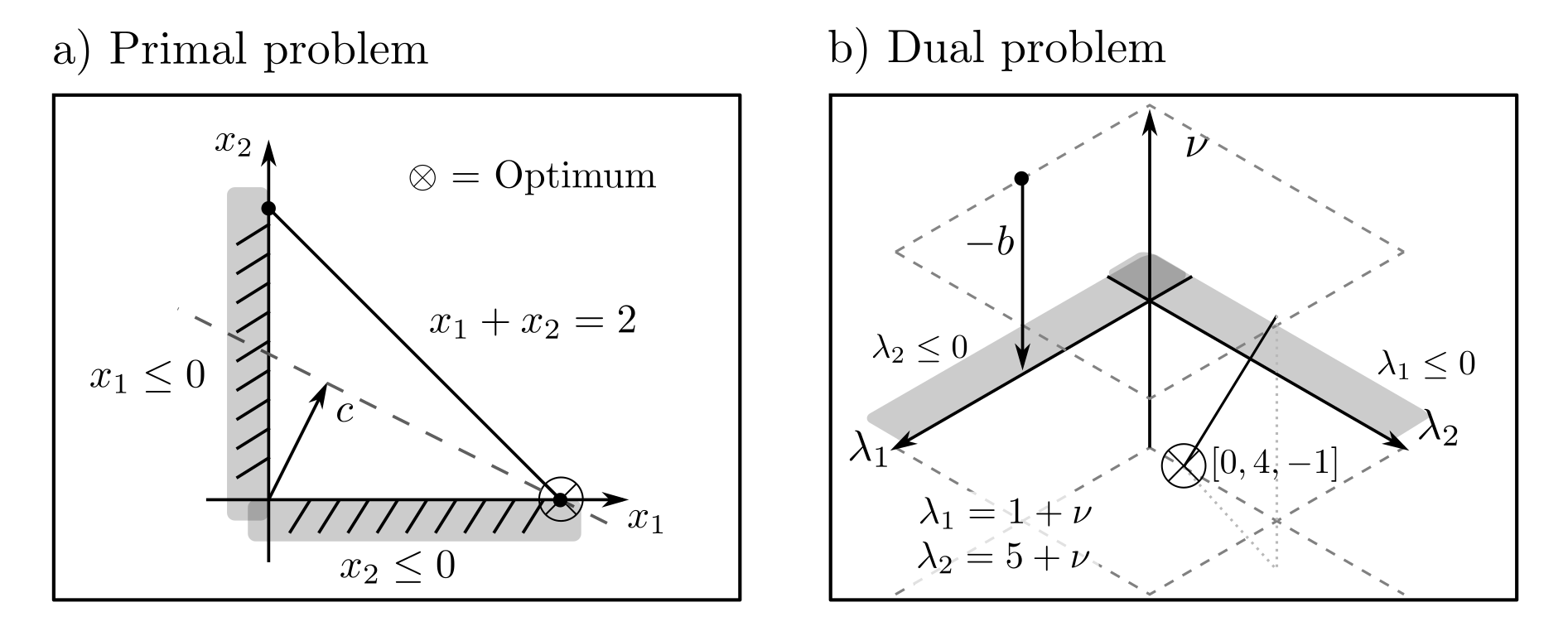
This can be demonstrated using the archetypal production example, which was also used to illustrate linear programming. Product quantities $x=[x_1,x_2]\ge 0$ should be produced to meet the demand of $x_1+x_2=2$ and minimize the costs $c^Tx = c_1x_1+c_2x_2$ with $c=[1,5]$ . The corresponding linear program

$\begin{align} P~~~~~~\min_x ~~~&c^Tx ~~~~~~~&c=[1,5] \\ \text{s.t.} ~~~&Ax =b &b=2 ~~~A=[1,1] \\ & x\ge 0 & \end{align}$

is solved by algorithms to $x^*=[2,0]$ with the minimal costs $c^Tx^*=2$ . The dual program

$\begin{align} D~~~~~~\max_{\nu,\lambda} ~~~&-b^T\nu \\ \text{s.t.} ~~~& A^T\nu +c -\lambda =0 \\ & \lambda \ge 0 \end{align}$

yields $g(\nu,\lambda)=\inf_x c^Tx+\nu^T(Ax‑b)-\lambda^Tx = \inf_x -\nu^Tb +(c^T+\nu^TA-\lambda^T)x$ , where the latter formulation either has the value $-\nu^Tb$ (if $c+A^T\nu — \lambda =0$ ) or $-\infty$ (in all other constellations).

Interpretation

The dual problem is also an LP and can be solved to $\nu^*=-1, \lambda^*=[0,4]$ with a maximum value $d^*=-b\nu^*=2$ . Two conclusions can be drawn from this:

The duality gap $p^*-d^*$ is $0$ . $P$ cannot have a solution $p^*$ with values less than 2 since $d^*=2$ is a lower bound. Since $p^*=d^*$ and there is only one optimum, it has been uniquely identified, and both optimization problems have been certifiably solved correctly.
The optimal parameters \nu^*, \lambda^* of the dual problem are [\nu^*]=-1 and [\lambda_1^*,\lambda^*_2]=[0,4]. They are directly related to the gains that would arise from disregarding the constraints [1, p.252].
- The solution of $P$ with the changed constraint $x_1\ge 1$ instead of $x_1 \ge 0$ is $x^*=[2,0]$ with $c^Tx^*=2$ — a change of size $\lambda_1^*=0$ of $p^*$ .
- The solution of $P$ with the changed constraint $x_2\ge 1$ instead of $x_2 \ge 0$ is $x^*=[1,1]$ with $c^Tx^*=6$ — a change of size $\lambda_2^*=4$ of $p^*$ .
- The solution of $P$ with the changed constraint $x_1+x_2=1$ instead of $x_1+x_2=2$ is $x^*=[1,0]$ with $c^Tx^*=1$ — a change of size $\nu^*=-1$ of $p^*$ .

Thus, $\nu^*, \lambda^*$ quantify the economic loss caused by the constraints and at what price avoiding them would be appropriately justified.

Application

If the primal program is an optimal production management problem, the dual program is a problem of optimal pricing by raw material suppliers [2, pp. 77–80]. Dual programs enable sensitivity analysis of the original problem and a better assessment of the constraints. They shift focus away from optimal decisions within the system and towards optimal system design. They represent interesting problems regardless of their relationship to the primal program.

When $p^*=d^*$ holds for the pair $(P,D)$ of problems, we speak of strong duality. Strong duality is linked to the fulfillment of Slater’s conditions concerning the feasible set of $P$ and is the standard case for LP, QP, QCQP, SOCP, and SDP. The relationships between $P$ and $D$ are exploited by primal-dual solution algorithms, which perform optimization steps for $P$ and $D$ synchronously and coupled. These methods are extremely popular due to the certifiability of the solution and the rapid convergence by utilizing primal and dual gradients [3, p. 115].

Sources

[1] Boyd, S., & Vandenberghe, L. (2004). Convex Optimization. Cambridge: Cambridge University Press.

[2] Vanderbei, Robert J. (2013). Linear Programming: Foundations and Extensions. USA: Springer US.

[3] De Klerk, E. (2006). Aspects of Semidefinite Programming: Interior Point Algorithms and Selected Applications. Berlin Heidelberg: Springer Science & Business Media.