Theory: Numerics and solver
Definition

Numerical analysis deals with the algorithmic computer-aided solution of specific problems in applied mathematics. The algorithms designed in numerical analysis lead in a finite number of steps from standardized problem formulations to an approximate solution.
The implementation of an algorithm for solving optimization problems in the form of executable program code is called a solver.
Simple brute-force approaches
Solution algorithms for problems of the form \(\min_x f(x) : x \in D\) are designed to generate a sequence \(x_1, …, x_m \in D\) such that \(f(x_m) — f(x^*) \le \epsilon\), where \(x^*\) is the true optimum and \(\epsilon\) is a small positive number specifying the minimum accuracy of the approximate solution \(x_m\).
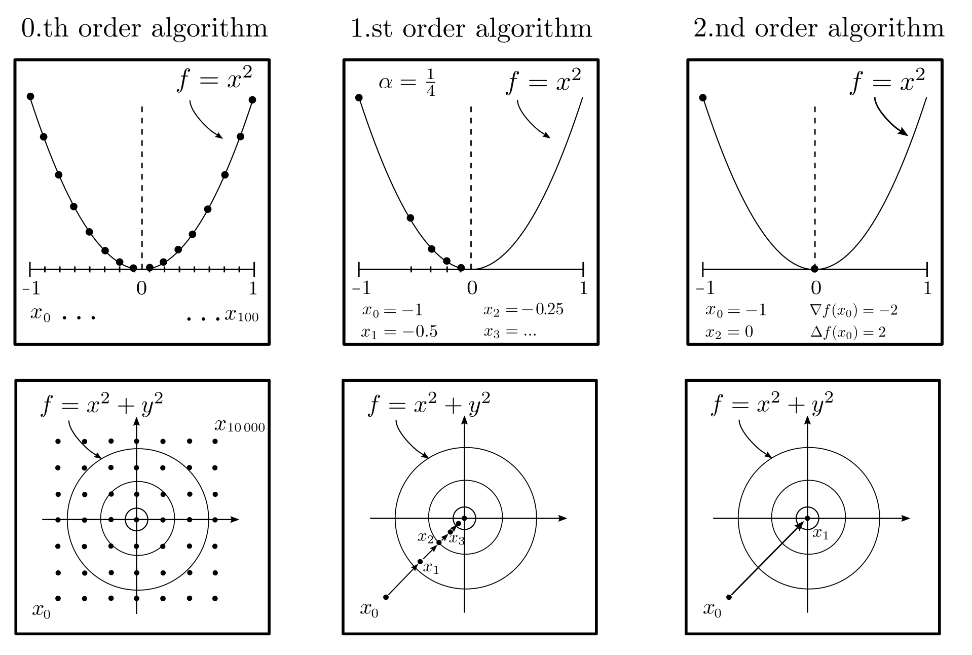
The solution algorithm requires access to the objective function \(f\) and the constraints \(D\). In the most general case, no global structural information is known, and only specific function values \(f(x_1), …, f(x_m)\) can be provided. With this sparse information, achieving an approximate solution \(x_m\) with \(f(x_m)-f(x^*)\le \epsilon\) requires at least [1, p. 11]
$$m \ge \left(\frac{L}{2 \epsilon} ‑1 \right)^n $$
optimization steps, where \(n\) is the number of dimensions of the optimization variable \(x\) and \(L\) is an upper bound for the derivative of \(f\). This equation shows that finding the optimal \(x^*\) by systematically trying different values of \(x\) is a futile endeavor: even for an \(x\) with 10 components, a standard computer would need several million years, and each additional dimension multiplies this time duration by a hundredfold [1, p. 12].
Simple derivative-based approaches
If both the function value \(f\) at the points \(x_1, x_2, …\), as well as the vector \(\nabla f\) of first derivatives (gradient) and the matrix \(\Delta f\) of second derivatives (Hessian matrix) are available, the number of optimization steps required is significantly reduced. Gradient-based methods
$$ x_{k+1} = x_k — \alpha \nabla f(x_k)~~~~~~k=0, 1, … ~~~~~\alpha >0 \text{ step size}$$
or the Newton method
$$ x_{k+1}= x_k — \Delta f^{-1}\nabla f ~~~~~~k=0, 1, …$$
typically have linear or quadratic convergence rates [1, p. 37]. This means that with each optimization step, the number of correct decimal places of \(x_k\) increases by a constant amount or doubles. The abovementioned problem, which is only solvable investing millions of years of computation time purely based on function values \(f(x_1), f(x_2), …\), is solved in a few milliseconds with the Newton method.

Conic optimization
The more is known about the function \(f\) to be minimized, the faster and more reliable the optimization works. It has been shown that information is best formulated in the form of cone conditions, so that all nonlinearities are embedded in the constraint \(x \in \mathcal{C}\), where \(\mathcal{C}\) is a convex cone. The optimization problem
\begin{align} \min_x & \langle x, c \rangle \\ \text{s.t.}& Ax = b \\ & x \in \mathcal{C} \end{align}
is called a cone program, and it has been proven that every convex optimization problem can be written in this manner [2, p. 60].

Solution procedures
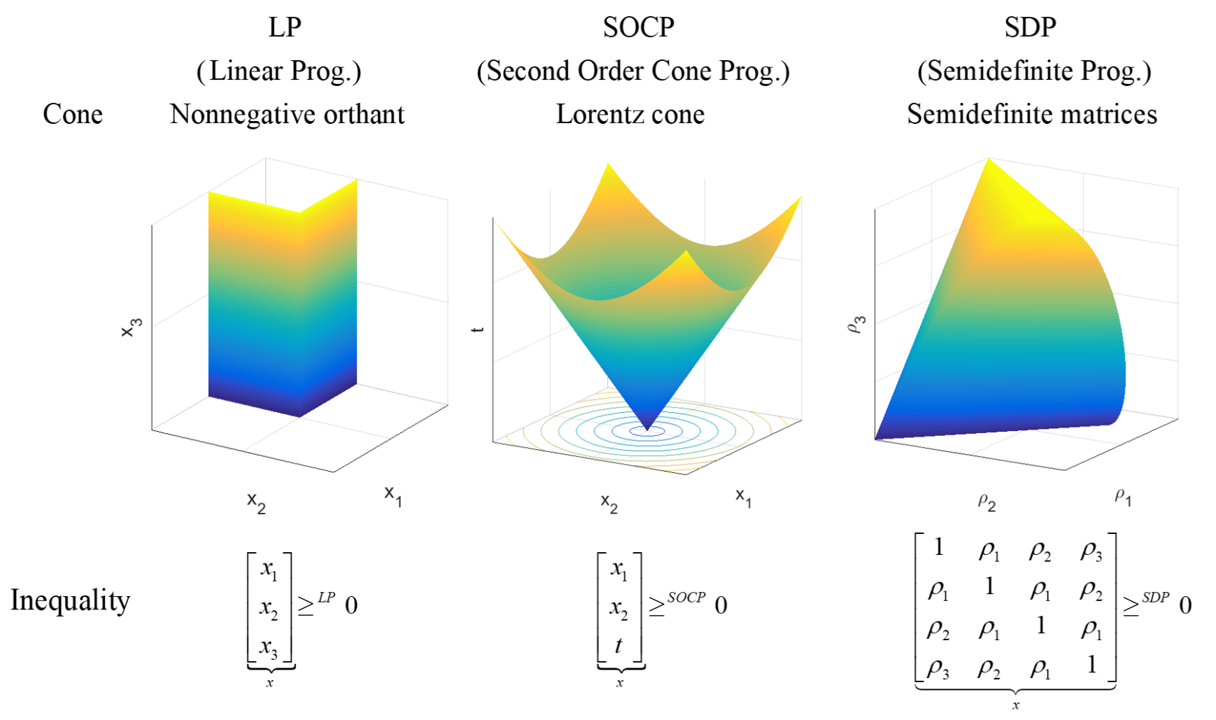
The class of cone programs is extremely expressive. Another advantage is that many cone programs (including LP, QP, QCQP, SOCP, SDP) can be efficiently solved.
This is done by replacing the constraints with logarithmic barrier functions, which tend towards infinity at the boundary of the feasible set; a sequence of unconstrained problems converging to the original problem with constraints is solved. The number of computational steps in the resulting methods depends polynomially on the dimension \(n\) of the problem and no longer exponentially [2, pp. 288–297].
To generate certifiably correct solutions, the original and dual problems are solved simultaneously by solving the primal-dual pair of optimization problems
\begin{align}
P ~~~ \min_X & \langle C,X\rangle_F \hspace{5cm} D ~~~ &\max_{y,S} & \langle b,y\rangle \\
\text{s.t.}& \langle A_k^T,X\rangle_F = b_k, ~~~ k=1, …, m_1 &\text{s.t.}& \sum_{k=1}^{m_1} y_k A_k + S = C \\
& X \succeq 0 && S \succeq 0
\end{align}
at the same time. Here, \(\langle C,X\rangle_F= \sum_{k=1}^n\sum_{l=1}^n C_{kl}X_{kl}\). The minimization of the duality gap \(\langle C,X \rangle_F — \langle b,y\rangle=\langle X,S\rangle_F\) then takes place using the logarithmic barrier function \(-(\log \det X + \log \det S)=-\log \det (XS)\) that tends towards infinity at the boundary of the positive semidefinite cones thereby leading to the optimization problem [3, p. 13]:
\begin{align}
\min_{X,y,S} ~~~&\langle X, S\rangle_F — \mu \log \det(XS) \\
\text{s.t.} ~~~ & \langle A_k^T, X\rangle_F = b_k ~~~~~ k=1, …, m_1 \\
& \sum_{k=1}^{m_1} y_k A_k + S = C
\end{align}
The resulting problem must be solved for a decreasing sequence of values for \(\mu\) to ensure convergence to the original problem’s solution.
Algorithms
The specific algorithm proceeds from feasible primal and dual variables \(X^0, S^0, y^0\) through the following steps until convergence [3, p. 118]:
\[
\begin{align}
X_{k+1} &= X_k + \Delta X, ~~~~~~ \Delta X = \mu_k S_k^{-1} — X_k — D\Delta S D \\
S_{k+1} &= S_k + \Delta S, ~~~~~~ \Delta S = \sum_{k=1}^{m_1} \Delta y_k A_k \\
y_{k+1} &= y_k + \Delta y, ~~~~~~ \Delta y = Q^{-1} g \\
\mu_{k+1} &= \alpha \mu_k, ~~~~~~ 0 < \alpha < 1
\end{align}
\]
Where \((Q)_{kl} = \langle D^T A_k^T, A_l D \rangle_F\), \(g = \mu \langle A_k^T, S_k^{-1} \rangle_F — b_k\), and \(D = S_k^{-1/2} (S_k^{1/2} X S_k^{1/2})^{1/2} S_k^{-1/2}\). As shown in the equations, forming and inverting large matrices is a part of the computation process. While computationally intensive, with modern computational capabilities this approach is still feasible for thousands of variables. Since LP, QP, etc., are only special instances of SDP, the optimization algorithm presented here is quite representative for approaches to other problems besides just semidefinite programming.
Solvers
In addition to some commercial solvers, there are also publicly available and free open-source solvers. For performance reasons, they are often written in the C programming language. We would like to particularly highlight the modeling framework CVXPY [4] for convex optimization problems. Although it is not a solver itself, it provides a unified interface to a variety of solvers and an automated grammar for formulating convex problems.
| Name solver | Licence | Capabilities | Organization / Reference |
|---|---|---|---|
| CVXOPT | GNU GPL | LP, QP, SOCP, SDP | Stanford CO Group |
| ECOS | GNU GPL‑3.0 | SOCP | Embotech GmbH |
| GLPK | GNU GPL | LP, MILP | Moscow Aviation Institute |
| MDPtoolbox | BSD‑3 | DP | Steven Cordwell |
| OR tools | Apache 2.0 | LP, MILP | Google |
| SCIP | ZIB Academic License | LP, MILP, MINLP, CIP | Zuse Institut Berlin |
| scipy | BSD | LP, Blackbox | scipy python package |
| SCS | MIT | LP, SOCP, SDP, ECP, PCP | Stanford CO Group |
| CPlex | kommerziell | LP, QP, nonconvex QP, SOCP, MIQP, MISOCP | IBM |
| Gurobi | kommerziell | LP, MILP, QP, MIQP, QCP, MIQCP | Gurobi |
| Mosek | kommerziell | LP, QP, SOCP, SDP, MINLP | Mosek |
LP = Linear Program, QP = Quadratic program, QCP = Quadratically constrainted program, SOCP = Second order cone program, SDP = Semidefinite program, ECP = Exponential cone program, PCP = Power cone program, CIP = Constraint integer program, DP = Dynamic programming, MI = Mixed integer, NLP = Nonlinear program
Sources
[1] Nesterov, Y. (2013). Introductory Lectures on Convex Optimization: A Basic Course. Berlin Heidelberg: Springer Science & Business Media.
[2] Nesterov, Y., & Nemirovskii, A. (1994). Interior-point Polynomial Algorithms in Convex Programming. Philadelphia: SIAM.
[3] De Klerk, E. (2006). Aspects of Semidefinite Programming: Interior Point Algorithms and Selected Applications. Berlin Heidelberg: Springer Science & Business Media.
[4] Diamond S., & Boyd S., (2016). CVXPY: A Python-embedded modeling language for convex optimization. Journal of Machine Learning Research, 17(83), 1–5.
