Theory: Custom solutions
Problem statement

Not every practically relevant optimization problem can be formulated as an LP, QP, etc., and solved with existing software. However, if the problem is convex or the goal is to improve an existing solution without claiming global optimality, there are still good chances. The development of custom algorithms is indispensable in such cases.
KKT conditions
Under the hypothesis that both the objective function \(f(x)\) and the inequalities are twice differentiable and convex, and the equations are affine, the solution to the optimization problem
$$\begin{align}
\min_x &~~~ f(x) \\
\text{s.t.}&~~~ (Ax)_k = b_k ~~~~~~~~~~~ k =1, … ‚m_1 \\
& ~~~ g_l(x) \le 0 ~~~~~~~~~~~~~ l=1, … ‚m_2
\end{align}$$
is uniquely defined by a set of equations. These are called Karush-Kuhn-Tucker (KKT) conditions and state that \(x^*, \lambda^*, \nu^*\) are optimal primal and dual optimization variables if the system of equations
$$\begin{align}
\nabla f (x^*) + \sum_{k=1}^{m_1} \nu_k^* \nabla (Ax^*)_k + \sum_{l=1}^{m_2}\lambda^*_l \nabla g_l(x^*) &=0 \\
(Ax^*)_k — b_k &=0 ~~~~~ k=1, …, m_1 \\
g_l(x^*) &\le 0 ~~~~~ l=1, …, m_2 \\
\lambda^*_l &\ge 0 ~~~~~ l=1, …, m_2 \\
\lambda^*_kg_l(x^*) &=0 ~~~~~ l=1, …, m_2
\end{align}$$
are satisfied [1, p. 244]. The five equations reflect the optimality condition concerning the objective function, the feasibility of the primal and dual variables, as well as a complementarity condition that couples dual variables and constraints.

Newtons method with constraints
In the KKT system, particularly the first and third rows are nonlinear, and finding a direct solution is challenging. As described in the section on numerics, inequalities can be replaced by barrier functions, and the nonlinear equation can be resolved using the Newton method. The updates for the primal and dual variables
$$x_{k+1}=x_k + \Delta x ~~~~ \lambda_{k+1}= \lambda_k + \Delta \lambda ~~~~ \nu_{k+1}= \nu_k+\Delta \nu $$
are derived from a sequence of equation systems for the search direction \((\Delta x, \Delta \lambda, \Delta \nu)\). The systems of equations are indexed by a sequence of numbers \(\mu_0, \mu_1, …\) approaching \(0\) and are given by [1, p. 610]:
$$\begin{bmatrix} \Delta f (x_k) + \sum_{l=1}^{m_2}\lambda_l\Delta
g_l(x_k) & \nabla g(x_k) & A^T \\
-\operatorname{diag}(\lambda)\nabla g^T(x_k) &
-\operatorname{diag}(g(x_k)) & 0 \\ A & 0& 0\end{bmatrix}
\begin{bmatrix} \Delta x \\ \Delta \lambda \\ \Delta \nu \end{bmatrix} = — \begin{bmatrix} \nabla f(x_k) + \nabla g(x_k)+ A^T \nu \\ -\operatorname{diag}(\lambda) g(x_k) — \mu_k \vec{1} \\ Ax‑b \end{bmatrix} $$
where \(\vec{1}=[1, …, 1]^T\) , \( g(x_k)=[ g_1(x_k), … g_{m_2}(x_k)]^T\), \(\nabla g(x_k) =[ \nabla g_1 (x_k), … ‚\nabla g_{m_2}(x_k)]\) with \(\nabla g_l\) being the gradient of \(g_l\) and \(\Delta g_l(x_k))_{ij}=(\partial_{x_i} \partial_{x_j} g_l)(x_k)\). The term \( \operatorname{diag(v)}\) is the matrix with entries of the vector \(v\) on the diagonal. Effective methods for solving the equation systems lead to search directions \((\Delta x, \Delta \lambda, \Delta \nu)\) and ultimately to the solution of the optimization problem associated with the KKT system.
Numeric stability
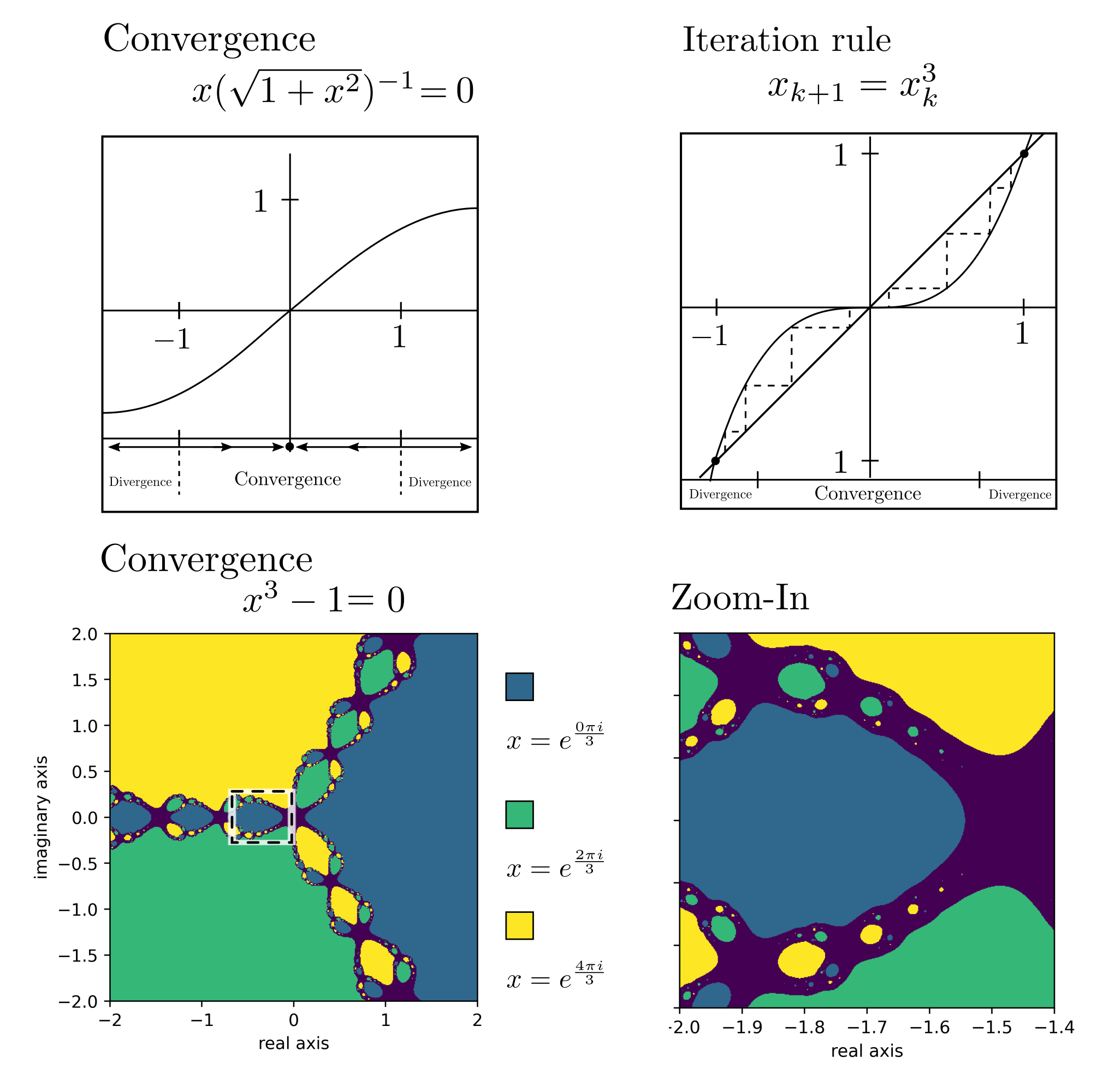
The above system of equations gives the impression of providing a complete and implementable scheme for convex optimization. However, this is not the case. In practice, additional steps must be taken to ensure numerical stability. Search directions must be scaled, centered, and corrected, among other adjustments [2]. Without these measures, the Newton method may face convergence issues. Additionally, in the presence of multiple local minima, the relationship between the starting point and the endpoint of the Newton method is far from obvious. See the following illustrations based on calculations from [3, p. 34] and [4, p. 21].

Example
Optimal estimation of correlations in data is essential for high-dimensional statistics related to stochastic processes. It can be considered as maximizing the likelihood of a Wishart-distributed random variable, ultimately leading to the optimization problem
\begin{align}
\min_{\gamma} & ~~~ \log \det C_{\gamma} + \langle S, C_{\gamma}^{-1} \rangle_F + r\left[- \log \det \gamma + \langle \operatorname{diag}(\lambda) ^{-1}, \gamma \rangle_F\right] \\
\text{s.t.} & ~~~ A \gamma =b \\
& ~~~ \gamma \succeq 0
\end{align}
[5, p. 193]. Here, \(\gamma\) is a positive semidefinite matrix of optimization variables, \(\langle \cdot, \cdot\rangle_F\) denotes the Frobenius inner product, \(S\) is an empirical covariance matrix, \(\lambda\) are eigenvalues, and \(C_\gamma\) is a covariance matrix constructed from \(\gamma\), with \(r\) being a regularization coefficient. The Newton steps are explicitly calculated as
\begin{align}
\gamma_{k+1} =& \gamma_{k}+\Delta \gamma_{1}- \gamma A^T(A\gamma A^T)^{-1}A\Delta \gamma_1 \\
&\text{ with } \Delta \gamma_1 = (1+r)^{-1}[(r‑1)\gamma +S_{\psi} — r\gamma \operatorname{diag}(\lambda)^{-1}\gamma] \\
& \text{ and } S_{\psi} \text{ a transformed covariance matrix}
\end{align}
and the optimization can be implemented, for example, in Python.

Implementation
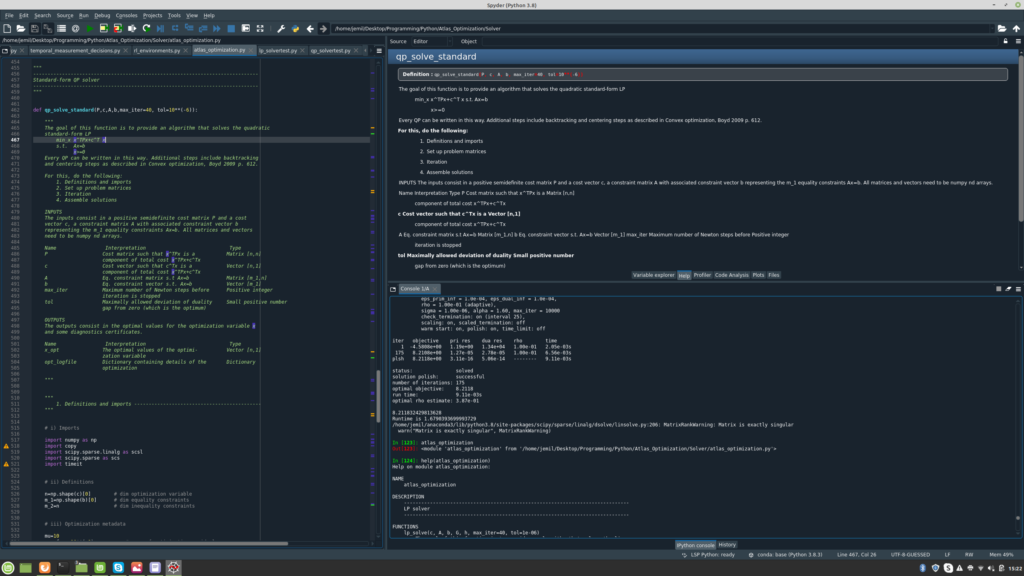
Practical implementations of a custom optimization algorithm require a reliable ecosystem of numerical programs. The Python programming language provides such an environment with NumPy [6] and is characterized by easy code interpretability and the availability of user-friendly graphical interfaces. This ease of entry is advantageous for both developers and clients.
Code & Sources
Example code: Theory_newton_convergence.py in our tutorialfolder
[1] Boyd, S., & Vandenberghe, L. (2004). Convex Optimization. Cambridge: Cambridge University Press.
[2] Mehrotra, S. (1992). On the implementation of a primal-dual interior point method. SIAM Journal on Optimization. 2 (4): 575–601.
[3] Nesterov, Y. (2013). Introductory Lectures on Convex Optimization: A Basic Course. Berlin Heidelberg: Springer Science & Business Media.
[4] Sternberg, S. (2014). Dynamical Systems. New York: Courier Corporation.
[5] Butt, J.A. (2019). An RKHS approach to modelling and inference for spatiotemporal geodetic data with applications to terrestrial radar interferometry. Dissertation ETH Zürich, Zürich.
[6] Harris, C.R., Millman, K.J., van der Walt, S.J., Gommers, R., Virtanen, P., Cornapeau, D., Wieser, E., Taylor, J., Berg, S., Smith, N.J., Kern, R., Picus, M., Hoyer, S., van Kerkwijk, M.H., Brett, M., Haldane, A., Fernandez del Rio, J., Wiebe, M., Peterson, P., Gerard-Marchant, P., Sheppard, K., Reddy, T., Weckesser, W., Abbasi, H., Gohle, C., & Oliphant T.E. (2020). Array programming with NumPy. Nature, Vol 585, No. 7825.
