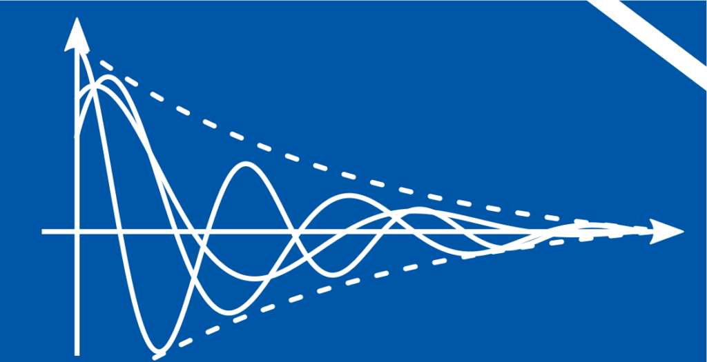
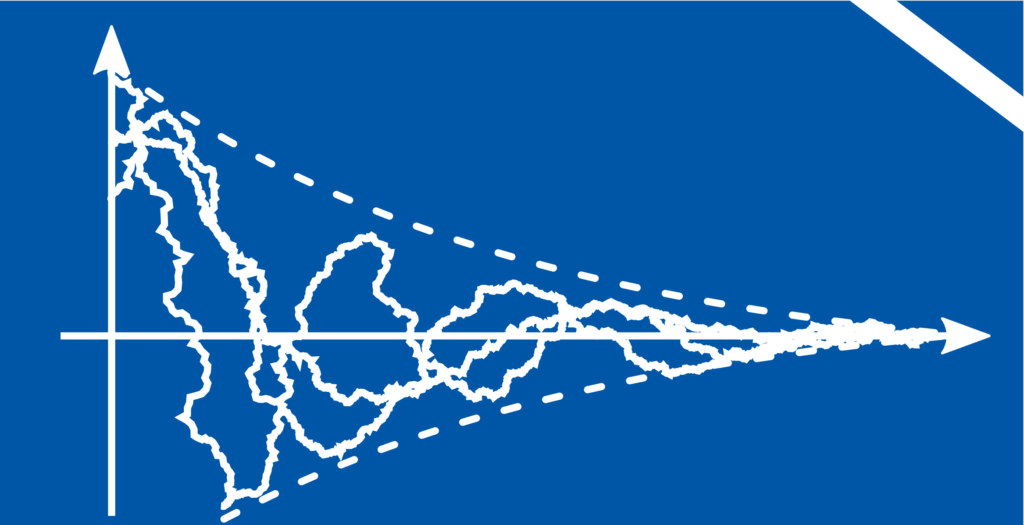
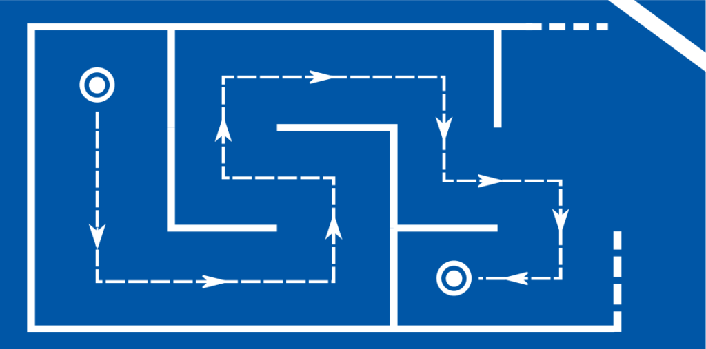
Optimal control - Atlas optimization

Optimal control: Overview

Definition

The term optimal control encompasses the theory and methods for the optimal control of systems. Control signals are to be chosen in such a way that a specific system state is achieved with minimal cost; optimal control often exhibits highly difficult problems due to its active and sequential nature.

Although the systems are often of a physical technical nature for historical reasons of development, they can also represent business management, economic, or information technology processes. The control signals are then, for example, dynamic resource flows, fiscal measures, or memory allocation rules. Common to all problem constellations is the goal of making optimal decisions under uncertainty.

Optimal control differs from optimal estimation and optimal design due to the presence of an opportunity for active control of the investigated system. Therefore, optimal control problems often have a temporal or at least sequential aspect, raising questions about the system’s dynamics and its controllability.

Example

A remote-controlled car is to be driven from position $x=0$ to position $x=1$ in time $T$. The acceleration $\ddot{x}$ can be influenced within certain limits by the control signal $u$. It should be chosen over the entire duration $T$ such that the total energy consumption $\sum_{t=0}^T \ddot{x}_t^2$ is minimized.

The optimization problem takes the form

$$ \begin{align} \min_{x_0, …, x_T, u_0, …, u_T} ~~~& \sum_{t=0}^T\ddot{x}_t^2 \\ \text{s.t.} ~~~& x_{t+1}=Ax_t+Bu_t\\~~~&x_0=[0,0,0]^T ~~~~~~~~~ x_T=[1,0,0]^T \\ ~~~& A=\begin{bmatrix} 1 & \Delta t & 0 \\ 0 & 1 & \Delta t \\ 0 & 0 & 1\end{bmatrix} ~~~~ B=\begin{bmatrix} 0 \\ 0 \\ \Delta t \end{bmatrix} \end{align}$$

Classes of problems

The above example is characterized by a high degree of predictability and requires precise knowledge of the dynamic relationships as well as an absence of random effects. In practice, this is not always the case, which is why formulations of the optimal control problem have also been developed for more complex situations.

Instead of a predefined plan $u_0, …, u_T$, current observations of the actual state must be incorporated into the control, resulting in a feedback loop [2, p. 102].

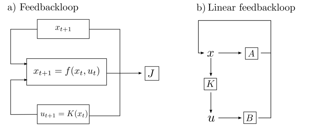
Then, the function $K(x_t)$ must be found such that $J$, as a measure of the inadequacy of the sequence $f(x_0,u_0), …, f(x_T,u_T)$, is minimized.

Class: Robust optimal control

Robust optimal control extends the optimization of control signals to situations where the relationship between system states $x_t$, control variables $u_t$, and the subsequent system state $x_{t+1}$ is not fully known.

In the above example, this corresponds to the case where, for instance, due to slippage or power transmission problems, the matrices $A$ and $B$ contain partially unknown elements [1, p. 428].

A control input $K(x_t) = u_t$ must then be found that satisfactorily controls the system
$$ x_{t+1} = Ax_t + Bu_t ~~~~~ A \in \mathcal{A}, B \in \mathcal{B} $$

regardless of the specific matrices $A \in \mathcal{A}$ and $B \in \mathcal{B}$. This amounts to the simultaneous satisfaction of several linear matrix inequalities and results in a semidefinite program.

Class: Stochastic optimal control

In stochastic optimal control, the system’s evolution is accepted as random, and instead of directly available system states $x_t$, only noisy observations are accessible.

For example, in the above example with the remote-controlled vehicle, if there were random uncontrollable effects such as wind or inaccuracies in signal transmission, then the system relationships could be described as follows.

$$ \begin{align} x_{t+1}&=Ax_t+Bu_t+w\\ y_t&=Cx_t+v \end{align}$$

Here, $x_t, A, B, u_t$ are as before, $y_t=Cx_t$ are the observations of the states, and $w$ and $v$ are random variables [1, p. 428], [3]. If only probabilities of state changes are known and possibly nonlinearities exist, then Markov decision processes can be used for problem formulation.

Class: Reinforcement learning

If neither dynamic relationships nor state transition probabilities are known, but the system to be controlled can in principle be simulated using a computer model, then reinforcement learning can be applied.

This situation, in the context of the above example with the remote-controlled car, would correspond to a scenario where no a priori information about the behavior of the system state and control input is available.

In reinforcement learning, the system behavior is instead empirically explored by executing control suggestions on a trial-and-error basis and observing their effects. This leads to a set of data used to train neural networks. Their task is to replicate an optimal function $u_t=K(x_t)$, which suggests the best action $u_t$ for each state $x_t$.

Due to the use of neural networks, the control inputs are of a nonlinear nature, and the approach is very data-hungry without guaranteeing optimality. However, this approach makes it possible to solve problems for which there is no hope with conventional methods. Examples include autonomous driving or the development of self-learning algorithms for the movement of robots or for controlling computer opponents in games [4].

Solutions

Depending on the class of the optimal control problem to be solved, it ranges from trivial to impossible to solve. Purely deterministic planning problems can often be solved through search algorithms or linear programming (LP). The presence of clearly defined random effects or model uncertainties requires the generation of stabilizing feedback loops and the minimization of error variances, necessitating the use of semidefinite programming (SDP). If no good process models are available, Markov decision processes can be used for stochastic modeling, or reinforcement learning is applied directly.

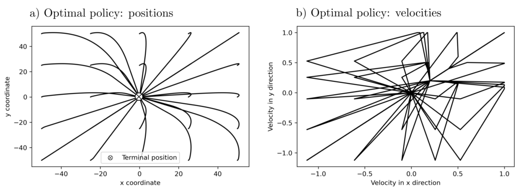
Iterative solution heuristics and individual examination of the proposed solutions are then inevitable. The methods are partly experimental and define the limit of what is currently achievable scientifically. A solution for an optimal control problem is then called a policy — a directive for every possible situation, indicating which behavior is optimal.

Applications

Optimal control offers countless application possibilities. These include technical applications such as the regulation of chemical reactions, control of robotic arms, or the coordination of harbor crane arms. Logistic problems such as adaptive traffic light control, adaptive scheduling of overtime, patient appointments, ambulance deployments, vehicle routing, and many issues from production planning and supply chain management.

The transition to financial or macroeconomic applications, such as the pricing of financial derivatives, stock portfolio management, and the control of economic activity levels, is seamless. Reinforcement learning is considered a practically applicable method of artificial intelligence. More examples can be found here.

In practical terms, there are many potential pitfalls with optimal control problems. Aside from the difficulty of formulating a specific goal as a convex optimality criterion, analyses must be conducted on how stable the developed controls are against random deviations. It is also not guaranteed that a desired state can be achieved using the available control options.

Code & Sources

Example code: OC_vehicle_control_1.py , OC_vehicle_control_2.py in our tutorialfolder.

[1] Wolkowicz, H., Saigal, R., & Vandenberghe, L. (2012). Handbook of Semidefinite Programming: Theory, Algorithms, and Applications. Berlin Heidelberg: Springer Science & Business Media.

[2] Anderson, B. D. O., & Moore, J. B. (2007). Optimal Control: Linear Quadratic Methods. New York: Courier Corporation.

[3] Balakrishnan, V., & Vandenberghe, L. (2003). Semidefinite programming duality and linear time-invariant systems. IEEE Transactions on Automatic Control, 48,(1), 30–41.

[4] Vinyals, O., Babuschkin, I., Czarnecki, W.M. et al. (2019). Grandmaster level in StarCraft II using multi-agent reinforcement learning. Nature, 575, 350–254.