Optimal estimation: Parameter estimation
Definition

Parameter estimation (also called regression) encompasses all those tasks that can be reduced to data-driven model fitting. The objective is to select parameters that bring the model behavior into the closest possible alignment with the actual observed real-world behavior.
It does not matter what the nature of the data is or the complexity of the model to be adjusted. For example, image classification can be considered a parameter estimation problem. In this case, the data consists of images annotated with image classes, and the model is a neural network with many parameters, which is intended to assign image classes to images. Thus, the transition to machine learning is seamless.
Example
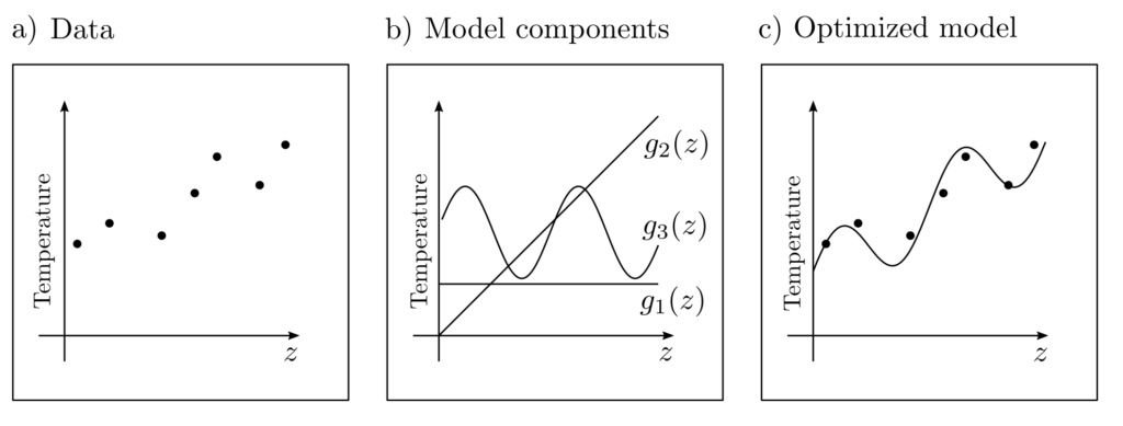
Suppose a weather station provides temperature readings \(l_k, k=1, … ‚n\) at regular intervals, leading to the sequence of measurements \( (l_1, z_1), … , (l_n, z_n)\), where \(z_k, k=1, … ‚n\) denotes the measurement times. Expecting long-term trends and periodic fluctuations due to time-of-day influences, the following model \(g(x,z) \) is proposed to explain the actual observed temperature data \(l\):
$$ \begin{align} l \approx g(x,z) = & x_1g_1(z) + x_2 g_2(z) + x_3 g_3(z) \\ & \underbrace{x_1}_{\text{Constant}} + \underbrace{x_2z}_{\text{linear trend}} + \underbrace{x_3\sin\left(\frac{2 \pi}{24}z \right)}_{\text{periodic influence}} \end{align}$$
In this model, the parameters \(x_1, x_2, x_3\) are undetermined and are to be chosen such that \(g(x,z_k)\) and \(l_k\) are approximately equal.

The solution to the optimization problem
$$ \begin{align} \min_x ~~~& \sum_{k=1}^n (l_k‑g(x,z_k))^2 \end{align}$$
is the optimal parameter vector \(x^*=[x_1^*, x_2^*, x_3^*]^T\). It allows interpretations of the relative strength of constant, linear, and periodic effects. The discrepancy \(\sum_{k=1}^n(l_k‑g(x^*,z_k))^2\) is an indicator of the overall suitability of the model.
Generalization
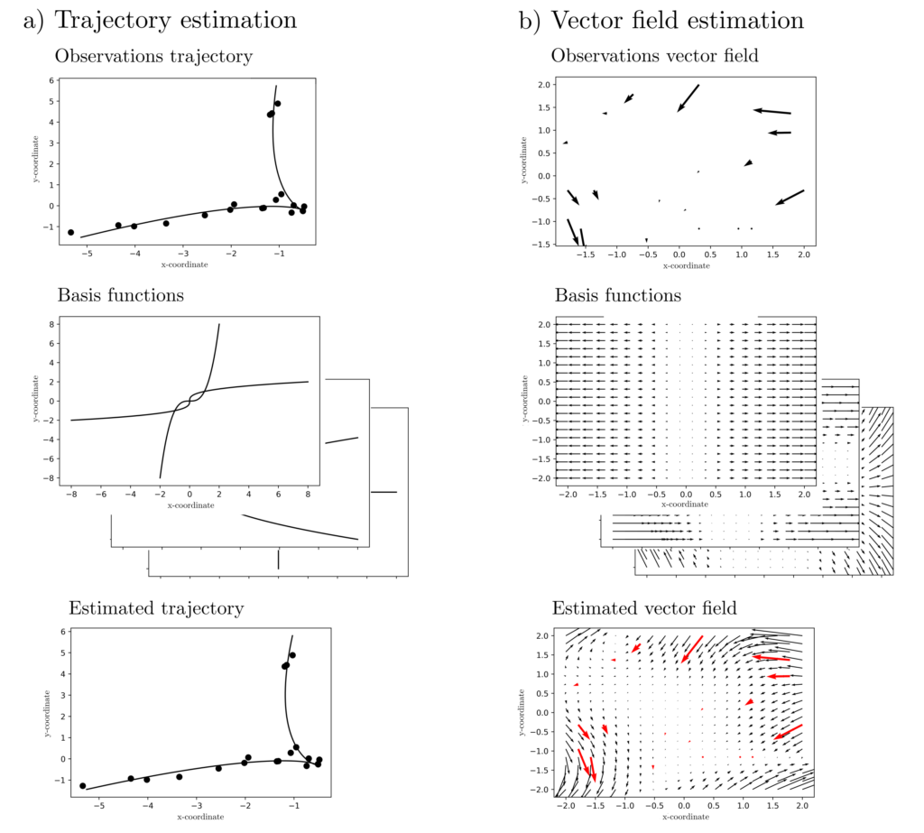
The approach above can easily be extended to data \(l_k\) of any dimension \(d_1\), function inputs \(z\) of any dimension \(d_2\), and any number of basis functions \(g_1(x,z), … , g_m(x,z)\). The optimization problem to determine the optimal parameters \(x^*\) is then formulated as:
$$ \begin{align} \min_x ~~~& \sum_{k=1}^n \|l_k-\sum_{j=1}^m x_jg_j(z_k)\|_2^2 \end{align}$$
where \(g(x,z)=\sum_{j=1}^m x_jg_j(z)\) is a function from \(\mathbb{R}^{d_2}\) to \(\mathbb{R}^{d_1}\) and \(\|v\|_2^2 = \sum_{k=1}^{d_1}v_k^2\) measures the length of the vector \(v\in \mathbb{R}^{d_1}\). In the form above, without additional constraints or complications, this is a quadratic program whose solution can be explicitly written as:
$$ \begin{align} x &=(G^TG)^{-1}G^T l \\ l&\in \mathbb{R}^{n d_1} ~~~~ l=[l_{11}, … , l_{1 d_1}, …, l_{n1}, …, l_{nd_1}]^T \\ G & \in \mathbb{R}^{n d_1} \times \mathbb{R}^{m} ~~~~ G=\begin{bmatrix} G_1 \\ \vdots \\ G_n \end{bmatrix} \\ G_k &\in \mathbb{R}^{d_1} \times \mathbb{R}^{m} ~~~~ G_k=\begin{bmatrix} g_{11}(z_k) & \cdots & g_{n1}(z_k) \\ \vdots & \ddots & \vdots \\ g_{1d_1}(z_k) & \cdots & g_{md_1}(z_k)\end{bmatrix} \end{align}$$
Here, \(g_{ij}(z_k)\) is the \(j-\)th entry of the vector \(g_i(z_k)\). This formulation allows solving parameter estimation problems for, e.g., two-dimensional trajectories and vector fields; see the illustration.

Interpretation
The previous formulations contain quadratic objective functions of the form \(\sum_{k=1}^n \|l_k‑g(x,z_k)\|_2^2\) and are thus least-squares problems. Minimizing these objective functions is sensible when the model class \(g(x,z)=\sum_{k=1}^m x_mg_m(z)\) can completely explain the data except for (standard) normally distributed residuals \(\epsilon\). Then it holds that
$$ l_k=g(x,z_k)+\epsilon_k \Leftrightarrow \epsilon_k= l_k‑g(x,z_k). $$
The probabilities of the residuals \(\epsilon_1, …, \epsilon_n\) are then \(p(\epsilon_k)= (2 \sqrt{\pi})^{-1} \exp\left( — \frac{1}{2} \epsilon_k^2\right)\). The probability of the occurrence of all residuals \(\epsilon_1, …, \epsilon_n\) together is
$$ p(\epsilon_1, …, \epsilon_n)=\prod_{k=1}^n p(\epsilon_k) = (2^n \pi^{n/2})^{-1} \exp\left( -\frac{1}{2} \sum_{k=1}^n \epsilon_k^2 \right)$$ for statistically independent residuals \(\epsilon_k \coprod \epsilon_j, k \neq j\). A choice of \(x\) such that all the residuals \(\epsilon_1= l_1‑g(x,z_1), …, \epsilon_n=l_n‑g(x,z_n)\) are as probable as possible leads to
$$ \max_x p(\epsilon_1, …, \epsilon_n) \Leftrightarrow \min_x \sum_{k=1}^n \left(l_k‑g(x,z_k)\right)^2. $$
The previous minimization problems can therefore be written as probability-maximizing estimators for the expected value of data \(l_k=g(x,z_k)+\epsilon_k\) under the assumption of uncorrelated, normally distributed noise \(\epsilon_k\).
Alternatives to least-squares
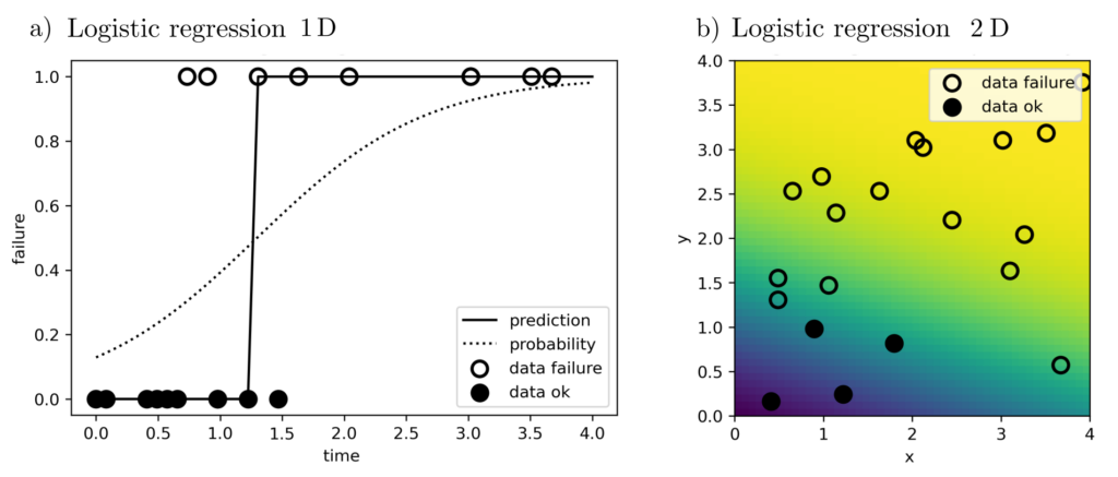
Not always is the assumption of normality realistic. The objective function and constraints may need to be adjusted to appropriately reflect the properties of the underlying data-generating processes. For example, the observed data might be binary indicator variables \(l \in \{0,1\}\), representing the failure of a component. If the failure probability needs to be estimated as a function depending on variables such as the component’s service duration, this leads to the logistic regression [1, p. 119] for the direct estimation of the cumulative probability distribution
$$p(\text{Component failure before time } t) = g(x,z)=[1+\exp(-x^Tz)]^{-1}$$
by maximizing the total probability \(\prod_{k=1}^n g(x,z_k)^{l_k}(1‑g(x,z_k))^{(1‑l_k)}\) of the failure observations \((l_1,z_1), … , (l_n,z_n)\). Multidimensional explanatory variables such as \(z=[\text{service duration, component price}]\) are also permissible and do not change the equations.

Applications and practical aspects
Classic least-squares parameter estimation is the workhorse of data analysis and modeling techniques. It is used wherever information needs to be extracted from data or models need to be adapted to real observations. It is easy to understand, well-researched, and allows for closed and simple-to-implement solution formulas. Therefore, it is widely used and any listing of specific applications would be grossly unrepresentative. Other parameter estimation approaches are less widespread but essential in cases involving non-normally distributed data.
From a practical standpoint, the challenge in formulating parameter estimation problems often lies in the stochastic modeling of the real-world process, which needs to be analyzed in terms of its probability distribution. Additionally, if the probability distributions are not from a specific parametric family, the probability-maximizing parameters may be difficult to find, as the associated optimization problem does not belong to one of the well-known classes such as LP, QP, SOCP, or SDP.
Code & Sources
Example code: OE_logistic_regression.py , OE_parameter_estimation_1.py , OE_parameter_estimation_2.py , OE_simulation_support_funs.py in our tutorialfolder
[1] Hastie, T., Tibshirani, R., & Friedman, J. (2013). The Elements of Statistical Learning: Data Mining, Inference, and Prediction. Berlin Heidelberg: Springer Science & Business Media.
