Optimal estimation : Estimation of failure probabilities
Problem statement

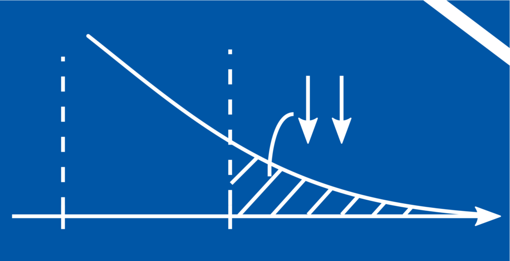
When production, formation, or measurement processes are characterized by uncertainties with a known probability distribution, the probabilities \(P(X \in C)\) can be directly calculated. Here, \(P(X \in C)\) describes the probability that a product, quantity, or measurement \(X\) takes values within the range \(C \subset \mathbb{R}\).
Analyzing such probabilities is an important diagnostic tool for systematically assessing decisions in uncertain situations when the impact of wrong decisions needs to be bounded even though some critical relevant information is unknown or subject to randomness.
Problem illustration
For example, if some machine components are manufactured whose lengths must lie within the interval \([a, b]\) for safe use, then the variations in component length caused by randomness in the manufacturing process pose a problem. It is necessary to examine the probabilities that:
- A component is manufactured with an incorrect length \(X \in C, C = \mathbb{R} \setminus [a, b]\)
- Due to measurement uncertainty, a correctly manufactured component is declared faulty (Type‑I error)
- Due to measurement uncertainties, a faulty manufactured component is declared correct (Type-II error).

If \(X\) is normally distributed with mean \(\mu\) and standard deviation \(\sigma\), then the probability \(P(X \in C)\) can be calculated as
$$P(X \le a) + P(X \ge b) = \int_{-\infty}^a p(x) \, dx + \int_b^{\infty} p(x) \, dx = 1 — \int_a^b p(x) \, dx = 1 — (\Phi(b) — \Phi(a)).$$
Here, \(\Phi(x)\) is the cumulative distribution function of \(X\) and can be found in mathematical reference books. Thanks to the one-dimensionality of this exemplary error estimation problem and the precise knowledge of the probability distribution, the problem can thus be solved with simple methods.
Chebychev inequality: Idea
In real applications, probability distributions are typically both high-dimensional and unknown, described only by descriptive statistical metrics such as empirical means and variances.
Nevertheless, even in these cases, worst-case probabilities \(P(X \in C)\) can be calculated by minimizing over probability distributions consistent with the observations \(E[X]=\mu \in \mathbb{R}^n\) and \(E[XX^T]=\Sigma \in \mathbb{R}^{n \times n}\). This allows for quantification of the probability that components do not meet quality requirements, naturally occurring objects exhibit atypical characteristics, or measurements produce grossly incorrect observations.
Chebychev inequality: Optimization formulation
The problem can be formulated as [1, p. 377]
$$ \begin{align} \min_{P,q,r} ~~~& \operatorname{tr} (\Sigma P) + 2 \mu^Tq+r \\ \text{s.t.} ~~~&x^TPx+q^Tx+r \ge 0 ~~\forall x \in \mathbb{R}^n \\ ~~~& x^TPx+q^Tx+r‑1 \ge 0 ~~ \forall x \in C \end{align}$$
where \(\Sigma\) and \(\mu\) are the problem data and the two inequalities ensure that the value of the optimization problem is an upper bound for \(P(X \in C)\). If \(C\) is the exterior of a polyhedron \(M\) defined by the \(n_c\) inequalities \(a_k^Tz \ge b_k, k=1, …, n_c\), then the infinitely many inequalities in the optimization problem above can be transformed into a requirement for the semidefiniteness of matrices. The equivalent semidefinite program is then [1, p. 377]
$$ \begin{align} \min_{P,q,r, \lambda} ~~~& \operatorname{tr} (\Sigma P) + 2 \mu^Tq+r \\ \text{s.t.} ~~~&\begin{bmatrix}P & q\\ q^T & r\end{bmatrix} \succeq 0 \\ ~~~& \begin{bmatrix} P & q \\ q^T & r‑1\end{bmatrix} \succeq \lambda_k \begin{bmatrix} 0 & a_k/2 \\ a_k^T/2 & ‑b_k \end{bmatrix} ~~~~ k=1, …, n_c \\ ~~~& \lambda_k \ge 0 ~~~~k=1, .…, n_c \end{align}$$
Chebychev inequality : Application
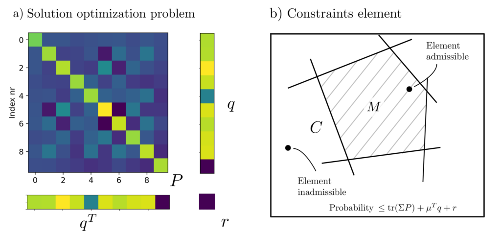
Das nachfolgende Bild illustriert eine beispielhafte Lösung des folgenden Problemes. Eine Maschinenkomponente mit zufälligen Längencharakteristiken \(X_1, …, X_{10}\) werde gefertigt. Die Erwartungswerte und Kovarianzen der Längencharaketeristiken sind bekannt; z.B. durch Messung einer Testmenge von Komponenten. Eine Komponente ist nur dann verwendbar zum Einbau in die übergeordnete Maschine, wenn sie die 20 Bedingungen
$ a_k^T x \le b_k ~~~~ k=1, …, 20$
an die Längen erfüllt. Dieses Problem ist leicht lösbar mit CVXPY [2].

The following images show the optimal matrices \(P\), vectors \(q\), and scalars \(r\) such that \(\operatorname{tr}(\Sigma P) + 2 \mu^Tq+r \) is the smallest upper bound for \(P(X\in C)\). With the \(P, q, r, \lambda\) shown there, \(P(X\in C)\le 0.4\). More information on this so-called moment problem can be found in [3, pp. 469–509].

Integration of additional information
If more is known about the underlying probability distribution than just the expected values \(E[X]\) and \(E[XX^T]\), this information can be used to improve error estimation and solve additional problems. Optimization over probability distributions can be enhanced through knowledge of:
Moment bounds \(M_k = E[X^k]\), for \(k = 1, \ldots, n\): Since the Hankel matrix $$\begin{bmatrix} M_0 & M_1 & M_2 & \cdots \\ M_1 & M_2 & \cdots & \\ M_2 & \vdots & \ddots & \\ \vdots & & & \end{bmatrix} \succeq 0$$ of the moments \(M_k\) of a probability distribution must be positive semidefinite, an optimization over moments can be written as an SDP [1, p. 171].
- Marginal probability distributions \(\bar{p} = \{\bar{p}_1, \ldots, \bar{p}_n\}\) and \(\bar{q} = \{\bar{q}_1, \ldots, \bar{q}_m\}\) of the random variables \(X_1\) and \(X_2\): The multivariate distribution is defined by the matrix $$P=\begin{bmatrix} p_{11} & \cdots & p_{1n}\\ \vdots & \ddots & \vdots\\ p_{m1} & \cdots & p_{mn}\end{bmatrix}$$ of probabilities \(p_{ij} = P(X_1 = x_i, X_2 = x_j) \ge 0\), allowing optimizations over multivariate probability distributions to be written as LPs with constraints \(\sum_{j=1}^n p_{ij} = \bar{q}_i\) and \(\sum_{i=1}^m p_{ij} = \bar{p}_j\).
- Cumulant-generating function \(\log E\left[ \exp(\lambda^T X)\right]\) of the probability distribution of \(X\)**: Depending on the precise form of this function, the Chernoff bound [1, p. 380] $$ \begin{align}P(X\in C) \le e^q ~~~~&~~~~ C=\{x: Ax \le b\} \\q= \min_{\lambda u} ~~~& b^Tu+\log E[\exp(\lambda^T X)] \\ \text{s.t.} ~~~&u \ge 0 ~~~ A^Tu+\lambda=0 \end{align}$$ results in an LP, QP, SDP, or a convex optimization problem not solvable by conventional methods to constrain the probability of an event’s occurrence.
Applications and practical aspects
Error estimations of the type described above are particularly helpful in risk limitation. When statements must be made about quantities only known by their probability distribution or uncertain measurements need to be translated into definitive decisions, these methods can provide real added value.
The risk limits depend not on the precise probability distribution but on the overall configuration of the problem. This relationship can be used to find a problem configuration that reduces the risk limits to an acceptable level.

The established 6 \(\sigma\) criterion for defining statistical quality targets in production management is similar to the above methods, albeit mathematically less involved. The gain obtained through higher complexity and increased stochastic modeling effort results in sharper, less conservative probability estimates.
Code & Sources
Example code: OE_bounding_probabilities.py in our tutorialfolder
[1] Boyd, S., & Vandenberghe, L. (2004). Convex Optimization. Cambridge: Cambridge University Press.
[2] Diamond S., & Boyd S., (2016). CVXPY: A Python-embedded modeling language for convex optimization. Journal of Machine Learning Research, 17(83), 1–5.
[3] Wolkowicz, H., Saigal, R., & Vandenberghe, L. (2012). Handbook of Semidefinite Programming: Theory, Algorithms, and Applications. Berlin Heidelberg: Springer Science & Business Media.
