Optimal estimation: Estimation of functions
Definition

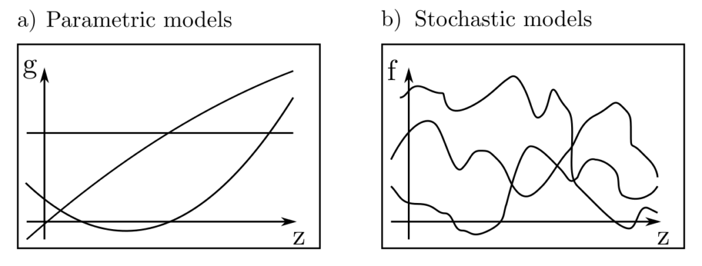
In parameter estimation, simplifying assumptions are made about the origin of observed data \(l\). They are considered explainable by a function \(g(x,z)\), which depends, among other factors, on parameters \(x\) with wrong model assumptions impacting estimation performance heavily.
In general function estimation, this simplifying assumption is abandoned, and the function \(f\) observed through data \(l\) is not restricted to a parametric family. Instead, \(f\) is considered as a stochastic process—a set of correlated random variables associated with locations \(t \in T\).
Relevance
Through this stochastic formulation, problems can be formalized and solved that are not accessible to normal parameter estimation. Additionally, stochastic processes provide a flexible functional model for \(f\) and allow the analysis of data for which no convincing parametric model of the form \(l = g(x, z)\) can be derived from external circumstances.
Some typical questions arise:
- Given measurements \(f(z_1), f(z_2)\), how large is \(f\) at other locations \(z\)?
- How likely is it that \(f(z_1)\ge 1\)?
- Given measurements \(f(z_1), f(z_2)\), what is \(\int_{0}^{1} f(z) dz\)?
- Are the data explainable by a smooth or an irregular, sharp-edged process?
Detailed explanation
For instance, if the data \(l_j, j=1, …, n\) are measurements of raw material deposits in the ground at locations \(z_j, j=1, …, n\), then all these questions are important for estimating the economic viability of mining the resources.
Indeed, the problem of interpolation—estimating all function values \(f(z)\) based on individual measurements \(l_j=f(z_j), j=1, …, n\)—was first systematically examined in the context of resource prospecting [1]. There are many functions \(f\) such that \(l_j=f(z_j), j=1, …, n\), thus the question arises as to which function \(f\) is most likely according to prior knowledge and data.
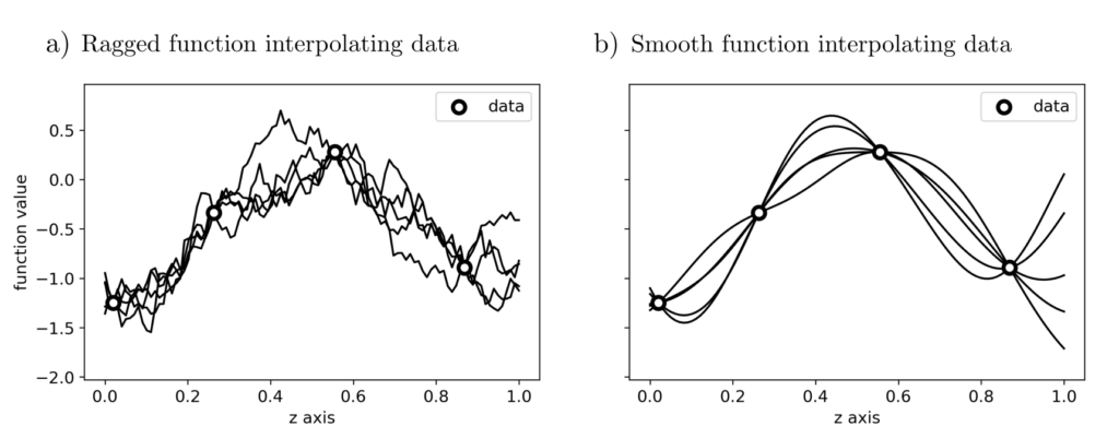
Interpolation: Optimization problem
The optimization problem for deriving the most probable function \(f\) is expressed as:
$$ \begin{align} \min_{f \in \mathcal{H}_K} ~~~& \|f\|_{\mathcal{H}_K}^2 \\ ~~~&\text{s.t.} f(z_j)=l_j ~~~~ j=1, …, n \end{align}$$
where \(\mathcal{H}_K\) is a function space and \(-\|f\|^2_{\mathcal{H}_K}\) indicates the probability of a function \(f\) within this space. Details of this formulation can be found in [2, p. 111]; particularly important is the reformulation as a quadratic program to determine weights \(\lambda \in \mathbb{R}^n\) with \(f(z)=\sum_{j=1}^n\lambda_j l_j\).
$$ \begin{align} \min_{\lambda} ~~~& (1/2)\lambda^TK_{II}\lambda — \lambda^TK_{I} \\ \text{s.t.} ~~~\sum_{j=1}^n \lambda_j =1 \end{align}$$
\(K_{II}\) and \(K_{I}\) are matrices and vectors containing the correlation structures of \(f\). They encode the underlying assumptions about, for example, the smoothness of \(f\). The optimization problem can be solved with solvers for quadratic programming or by hand.
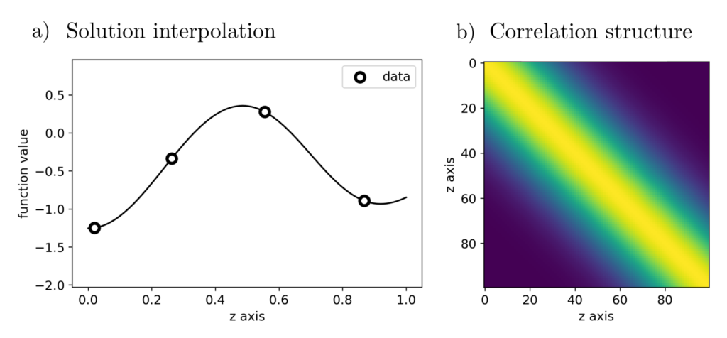
Correlation structure
The correlation matrices indicate how strongly the values \(f(z_1), f(z_2)\) at different positions \((z_1, z_2)\) are correlated: A value of \(0\) for \(z_1=0\) and \(z_2=1\) thus indicates that there is no significant correlation between \(f(0)\) and \(f(1)\). If there are no reliable prior assumptions about the correlation structures, they can also be derived from the data. This too is an optimal estimation problem and can be reviewed here .
Abstract splines
Interpolating data is often helpful. However, data does not always arise from point measurements, is error-free, or its correlation structure is known. The currently most general, still efficiently solvable estimation problem is formulated as follows [2, p. 117]:
$$ \begin{align} \min_f ~~~& \|Af‑l\|^2_{\mathcal{H}_A}+ \|Bf\|^2_{\mathcal{H}_B} & \\ & f : \text{ Function to be estimated} && l : \text{ Data} \\ & A : \text{ Measurement operator} && \mathcal{H}_A : \text{ Function space of potential measurements} \\ & B : \text{ Energy operator} && \mathcal{H}_B : \text{ Function space of potential energies} \end{align}$$
Solutions to these minimization problems are called abstract splines and they maximize the probabilities of discrepancies \(Af‑l\) between actual and hypothetical observations as well as the probability of \(f\) itself. The measurement operator \(A\) maps functions \(f\) to hypothetical observations \(Af\) and the energy operator \(B\) maps functions \(f\) to quantities \(Bf\), whose probability distribution is known.
Applications
The solutions to a vast number of optimal estimation problems can be represented as abstract splines. For instance, if \(f\) is a two-dimensional function and \(Af\) are line integrals \( (Af)_j= \int_{z_0}^{z_j} f(z) dz\), then the abstract splines are solutions for tomography problems, as shown in the figure.
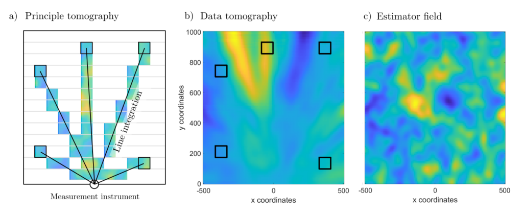
If, however, \(A\) is simply the identity operator and \(\mathcal{H}_A\) and \(\mathcal{H}_B\) are function spaces of functions with different correlation structures, then the abstract splines represent solutions for signal separation problems.
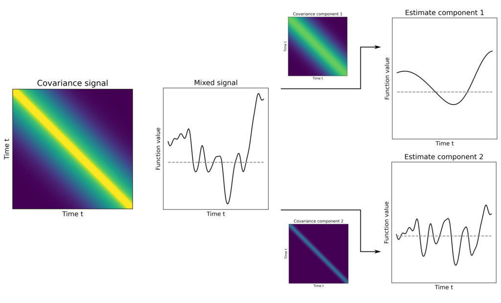
In addition to these two examples from signal processing, optimal function estimation is also used for many other purposes. Applications include raw material prospecting, image processing, measurement data evaluation, modeling environmental phenomena concerning e.g., epidemiological spread processes, distribution of atmospheric parameters, geological properties, and land use, as well as creating surrogate models, compressing and filtering video data, and much more.
Practical aspects
Formulating and solving real-world problems as abstract function estimation problems involves several steps. Firstly, there’s the challenge of identifying a specific task as solvable by estimating a function, which is not always straightforward. Furthermore, precise formulation and transformation play a crucial role in ensuring the solvability of the optimization problem. Strictly speaking, abstract splines are optimization problems in infinite-dimensional spaces (function spaces typically have this property); hence, clever manual computations are required.
Lastly, the correlation structures of the solutions must either be prescribed based on previous data foundations or based on prior assumptions. This requires experience in modeling with stochastic processes. If these three challenges are successfully mastered, the result is an estimation that is optimal from a stochastic perspective.
Code & Sources
Example code: OE_conditional_simulation.py , OE_random_quantities.py , OE_functional_signal_separation.py , OE_simulation_support_funs.py in our tutorialfolder
[1] Cressie, N. (1990). The origins of kriging. Mathematical geology, 22, 239–252.
[2] Berlinet, A., & Thomas-Agnan, C. (2011). Reproducing Kernel Hilbert Spaces in Probability and Statistics: . Berlin Heidelberg: Springer Science & Business Media.
