Optimal control: Robust optimal control
Problem statement

In robust optimal control, the goal is to stabilize a system whose exact dynamic properties are unknown and can only be constrained to a specific uncertainty range. Additionally, the state of the system may only be partially observable.
Trotzdem soll ein zeitabhängiger Input \(u(t)\) gefunden werden, der den Systemzustand \(x(t)\) stabilisiert, d.h. \(\lim_{t\rightarrow \infty} x(t)=0\) unabhängig von der eigentlichen Dynamik. Probleme dieser Art treten z.B. bei der Steuerung von Drohnen [1], Helikoptern, Festplattenauslesealgorithmen [2] und generell sobald die Steuerungsmechanismen eines Systems Unsicherheiten aufweisen.
Optimal control for uncertain dynamics
The dynamics of a system with partially unknown dynamics are given by the equation
$$ \dot{x}(t) = Ax(t) + Bu(t) ~~~~~~[A,B] \in Co([A_1,B_1], …, [A_n,B_n]), $$
which couples system changes \(\dot{x}\) with the time-dependent state variables \(x(t)\) and control inputs \(u(t)\). The matrices \(A\) and \(B\) are to represent all possible weighted averages \([\sum_{k=1}^n\lambda_k A_k, \sum_{k=1}^n \lambda_k B_k], \sum_{k=1}^n\lambda_k=1, \lambda_k \ge 0\) among the corner points \([A_1, B_1], …, [A_n, B_n]\); this set is also called the convex hull \(Co\). If \(A\) and \(B\) were known constant matrices, it would be a classic planning problem.
A system \(\dot{x}=Ax\) is stable if there exists a quadratic function \(V(x)=x^TPx, P\succeq 0\) such that [3, p. 428]
$$\dot{V}(x) = x^T(A^TP+PA)x <0.$$
This so-called Lyapunov function proves that there is an energy function that explains all trajectories that can be generated by the system. A feedback matrix \(K\) with \(u(t)=Kx(t)\) is sought, which stabilizes the system. It can be derived to \(K=YQ\) from the solutions \(Q, Y\) of the following semidefinite system of equations for the matrices \(Q\) and \(Y\) [3, p. 428].
$$ Q=Q^T \succ 0, ~~~~~~~~~ (QA_i^T+A_iQ)+(Y^TB_i^T+B_iY) \prec 0~~~~i=1, …,n$$
Example: Harmonic oscillator
The following example illustrates the application and approach. A vibrating system is mass-produced and used in different situations. Although the dynamics vary depending on the situation, a single, universally valid feedback control for vibration damping is to be used.
Let \(s\) be the spatial variable, and as usual, dot and double dot denote the first and second time derivatives, respectively. A harmonic oscillation is characterized by the differential equation
$$ \begin{align}\dot{s} & = — \omega s \\ x&=\begin{bmatrix} s \\ \dot{s} \end{bmatrix} \\ & \Rightarrow \dot{x}=\begin{bmatrix} \dot{s} \\ \ddot{s} \end{bmatrix} =\begin{bmatrix} \dot{s} \\ — \omega s \end{bmatrix} = \begin{bmatrix} 0 & 1 \\ -\omega & 0 \end{bmatrix} \begin{bmatrix} s\\ \dot{s} \end{bmatrix}= Ax. \end{align}$$
Here, \(\omega >0 \) and the resonance frequency \(\sqrt{\omega}\) may vary depending on the situation. Suppose \(\omega\) lies between \(1/2\) and \(3/2\) and the control input is an acceleration; \(Bu=[0,0,u]^T\) with \(B=[0,0,1]^T\). Then the following SDP needs to be solved.
$$ \begin{align} \min_{Q,Y} ~~~& \operatorname{tr} (Q) \\ \text{s.t.} ~~~&Q \succ 0 ~~~~ \operatorname{tr} Q \ge 1 \\ &(Q A_1^T +A_1Q)+(Y^TB^T + BY) \prec 0 \\ &(Q A_2^T +A_2Q)+(Y^TB^T + BY) \prec 0 \\ & A_1 =\begin{bmatrix} 0 & 1 \\ ‑1/2 & 0 \end{bmatrix} ~~~~~~~A_2=\begin{bmatrix} 0 & 1 \\ ‑3/2 & 0\end{bmatrix} \end{align}$$
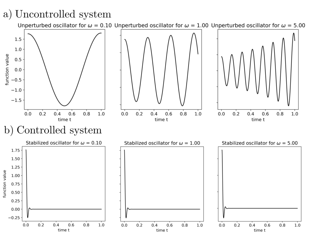
This semidefinite program can, for example, be solved with CVXPY [4] to \(K\approx [-60,-9]^T\). The effect of this feedback matrix can be seen in the figure below.

It is evident that the above control stabilizes the systems regardless of the exact natural frequencies. The trivial control \(u=-s\), for example, does not achieve this.
Unknown state and time-dependent dynamics
In a system to be controlled, if the time-dependent state \(x(t)\) can only be detected through an output signal \(y(t)=C_yx(t)\), and the dynamics
$$ \dot{x}=A(t)x(t)+Bu(t) ~~~~~~~A(t) \in Co([A_1, …, A_n]) $$
are time-varying, then the system is stabilizable only under certain conditions. The matrix \(A(t)\) is a time-varying linear combination $$A(t)=\sum_{k=1}^n\theta_k(t)A_k ~~~~\sum_{k=1}^n \theta_k(t)=1, \theta_k(t)\ge 0.$$ It is an element of the convex hull \(Co([A_1, …, A_n])\), describing the relationship between system changes \(\dot{x}\) and the system state \(x\). The indirectly observed state \(x\) is to be stabilized.
Such problems occur in systems that need to be maintained stably across a wide range of situations and whose description includes nonlinear terms and unobserved conditions [5]. This class of problems includes the development of autopilots for aerospace systems and the optimal control of chemical reactions in process engineering [6].
SDP formulations
Assuming that the mixing coefficients \(\theta_k(t)\) are known at any time, it can be shown that a stabilizable higher-dimensional embedding of \(x\) exists if the semidefinite system of equations
$$\begin{align} &\begin{bmatrix} S & I \\ I & R \end{bmatrix} \succeq 0 \\ &N_R^T(A_kR + R A_k^T)N_R \prec 0 ~~~~ k=1, …, n \\ &N_S^T(A_kS + S A_k^T)N_S \prec 0 ~~~~ k=1, …, n \end{align}$$
has a solution \(S, R\) [3, pp. 428–431]. Here, \(N_R^T\) and \(N_S^T\) are matrices whose columns form the basis of the null spaces of \(B^T\) and \(C_y\), respectively. More details can be found in [7, pp. 22–23]. If the system of equations is solvable, then the system
$$\begin{bmatrix} x \\ x_c \end{bmatrix} =\left( \underbrace{\begin{bmatrix} A(t) & 0 \\ I & 0\end{bmatrix}}_{\mathcal{G}} + \underbrace{\begin{bmatrix} 0 & B \\ I & 0 \end{bmatrix}}_{\mathcal{B}} \underbrace{\begin{bmatrix} A_c(t) & B_c(t) \\ C_c(t) & D_c(t) \end{bmatrix}}_{\Omega(t)} \underbrace{\begin{bmatrix} 0 & I \\C_y & 0 \end{bmatrix}}_{\mathcal{C}}\right) \begin{bmatrix}x \\ x_c \end{bmatrix}$$
can be solved for the unknown closed loop state transition matrix \(A_{cl}(t)=\mathcal{G}+\mathcal{B}\Omega(t) \mathcal{C}\). Furthermore, the condition \(A_{cl}^T(t)P+PA_{cl}(t) \prec 0 ~~~~~ P \succ 0 \)
can be satisfied, ensuring the system is stable since it dissipates energy along all possible trajectories. Solving the system of equations for each \(k=1, …, n\)
$$\begin{align} &(\mathcal{G}_k+\mathcal{B}\Omega_k\mathcal{C})^TP + P(\mathcal{G}_K + \mathcal{B}\Omega_k \mathcal{C}) \prec 0 \\ &P=\begin{bmatrix} S & (S‑R^{-1})^{1/2} \\ (S_R^{-1})^{1/2 T} & I \end{bmatrix} ~~~~~~\mathcal{G}_K=\begin{bmatrix} A_k & 0 \\ 0 & 0 \end{bmatrix}\end{align}$$
for \(\Omega_k\) results in a time-dependent overall solution through a weighted linear combination of the individual solutions for \(\Omega_k\). The system
$$ \begin{bmatrix} \dot{X} \\ \dot{X}_c \end{bmatrix} = \left( \begin{bmatrix} \sum_{k=1}^n \theta_k(t) A_k & 0 \\ 0 & 0 \end{bmatrix} + \begin{bmatrix} 0 & B \\ I & 0 \end{bmatrix} \left(\sum_{k=1}^n \theta_k(t) \Omega_k \right) \begin{bmatrix} 0 & I \\ C_y & 0 \end{bmatrix}\right) \begin{bmatrix}x \\ x_c \end{bmatrix}$$
is stable. The control input \(u\) derived from the output \(y\) is thus given by \(u(t)\) with
$$\begin{align} u(t) &= \sum_{k=1}^n \theta_k(t) C_c^kx_c + \sum_{k=1}^n \theta_k(t) D_c^ky \\ \Omega_k&=\begin{bmatrix} A_c^k & B_c^k \\ C_c^k & D_c^k\end{bmatrix} \end{align}$$
where \(x_c\) evolves according to \(\dot{x}_c = \sum_{k=1}^n A_c^kx_c+\sum_{k=1}^n\theta_k(t) B_c^kC_yx\).
Example: Circuit
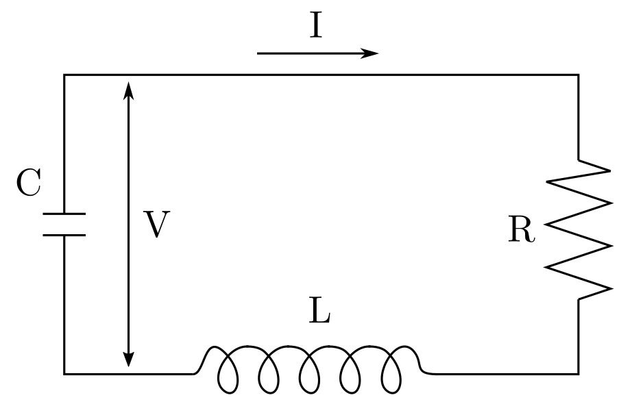
An example illustrates the approach. Consider a circuit with a resistor, an inductor, and a capacitor. According to [8, pp. 10–11], the relationship between voltage \(V\), current \(I\), and time \(t\) is given by the vector-valued differential equation

$$ \begin{bmatrix} \dot{V} \\ \dot{I}\end{bmatrix} = \begin{bmatrix}0 & — 1/C \\ 1/L & ‑R/L\end{bmatrix} \begin{bmatrix} V\\ I \end{bmatrix} + \begin{bmatrix} u_1 \\ u_2 \end{bmatrix} $$
where \(R\) is the resistance, \(L\) is the inductance of the coil, and \(C\) is the capacitance of the capacitor. We assume that:
- The change in voltage and current can be controlled via the control input \([u_1,u_2]^T\).
- \(C\) and \(L\) vary between 1 and 10.
- Only the current is observable, and the voltage is not measured.
Despite the problematic conditions 2. (variable circuit parameters) and 3. (voltage not observable), the system is to be stabilized. We apply the equations presented above and obtain the following chain of semidefinite systems of equations, which we can solve, for example, with CVXPY.
$$\begin{align}1.~~~~ \text{find} & ~~~R, S \\ s.t. &~~~ \begin{bmatrix} R & I \\ I &S \end{bmatrix} \succeq 0 \\ &~~~ \begin{bmatrix} 1 & 0\end{bmatrix} (S A_k + A_k^TS) \begin{bmatrix} 1 \\ 0 \end{bmatrix} <0 ~~~~~~k=1, …, 4 \\ &~~~ A_1=\begin{bmatrix} 0 & ‑1 \\ 1 & ‑R\end{bmatrix} ~~~~~A_2=\begin{bmatrix} 0 & ‑0.1 \\ 1 & ‑R\end{bmatrix} \\ & ~~~A_3=\begin{bmatrix} 0 & ‑1 \\ 0.1 & ‑0.1R\end{bmatrix}~~~~~A_4=\begin{bmatrix} 0 & ‑0.1 \\ 0.1 & ‑0.1R\end{bmatrix}\\2.~~~~ \text{find} & ~~~\Omega_k \\ s.t. &~~~(\mathcal{G}_k + \mathcal{B}\Omega_k \mathcal{C})^TP+P(\mathcal{G}_k+\mathcal{B}\Omega_k\mathcal{C}) \prec0 \\ & ~~~\mathcal{G}_k= \begin{bmatrix} A_k & 0 \\ 0 & 0\end{bmatrix} ~~~~~\mathcal{B}=\begin{bmatrix} 0& 0& 1&0\\0&0&0&1\\1&0&0&0\\0&1&0&0\end{bmatrix} ~~~~~\mathcal{C}=\begin{bmatrix} 0&0&1&0\\ 0&0&0&1\\ 0&1&0&0\end{bmatrix} \end{align}$$
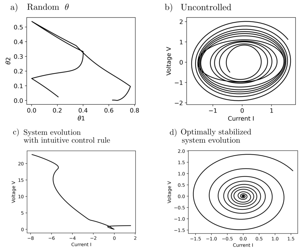
The result is visible in the figure below.

Indeed, the system is stable. This is not the case if the control input is chosen according to intuitive, manually conceived rules or left to itself. Therefore, the approach to optimal control of only partially observed systems with partially unknown dynamics provides real added value.
Code & Sources
Example code: OC_harmonic_oscillator_3.py , OC_harmonic_oscillator_4.py in our tutorialfolder.
[1] AlSwailem, S.I. (2004). Application of Robust Control in Unmanned Vehicle Flight Control System Design. Dissertation Cranfield University, Cranfield.
[2] Postlethwaite, I., Turner, M. C., Guido, H. (2007). Robust Control Applications. Annual Reviews in Control, 31, (1), 27–39
[3] Wolkowicz, H., Saigal, R., & Vandenberghe, L. (2012). Handbook of Semidefinite Programming: Theory, Algorithms, and Applications. Berlin Heidelberg: Springer Science & Business Media.
[4] Diamond S., & Boyd S., (2016). CVXPY: A Python-embedded modeling language for convex optimization. Journal of Machine Learning Research, 17(83), 1–5.
[5] Leith, D. J., & Leithead, W. E. (1998). Appropriate realisation of MIMO gain-scheduled controllers. International Journal of Control, 70, (1), 13–50.
[6] Klatt, K. U., & Engel S. (1998). Gain-scheduling trajectory control of a continuous stirred tank reactor. Computers & Chemical Engineering, 22, 491–502.
[7] Boyd, S., El Ghaoui, L., Feron, E., & Balakrishnan, V. (1994). Linear Matrix Inequalities in Systems and Control Theory. Philadelphia: SIAM Studies in Applied and Numerical Mathematics.
[8] Scheinerman, E. R. (2013). Invitation to Dynamical Systems. New York: Courier Corporation.
