Optimal control: Systems analysis
Problem statement

Controlling time-dependent systems is a challenging endeavor, and success cannot be guaranteed under all circumstances. Some systems are intrinsically unstable and can spiral out of control regardless of the control input.
Other systems do not provide the decision-making algorithm with enough information to derive meaningful control instructions.
To estimate the success of control, it is necessary to examine key system characteristics such as stability, controllability, and observability. Only then can the potential problems in controlling the system be identified, and limits of validity as well as guarantees of success be established. In practice, this theoretical system analysis is further complicated by unknown dynamic relationships that must be derived from observational data and preliminary considerations before any further investigation.
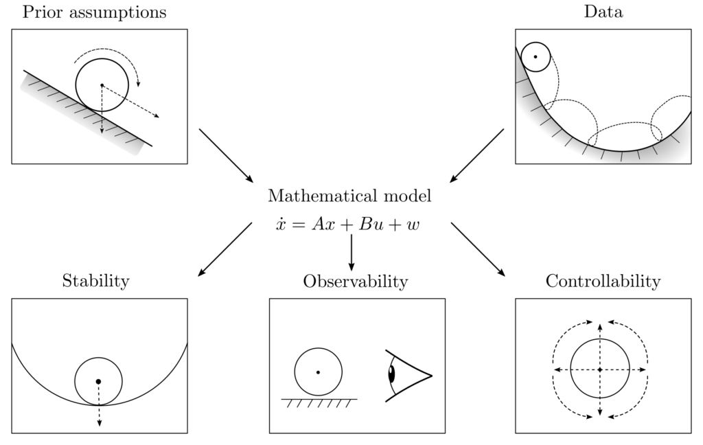
Exemplary system behavior
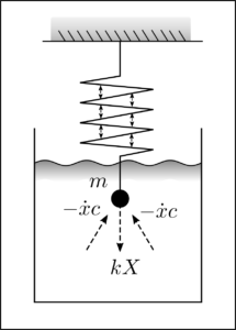
The given equation describes a damped harmonic oscillator:
$$ \ddot{x} + \frac{c}{m} \dot{x} + \frac{k}{m}x = 0 $$
This equation models the position \(x\), velocity \(\dot{x}\), and acceleration \(\ddot{x}\) of an elastically oscillating mass \(m\) in a typically viscous fluid with a damping coefficient \(c\). The parameter \(k\) is the spring constant, which couples the displacement and acceleration.
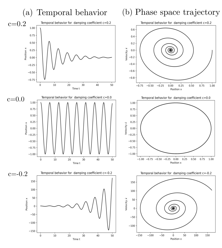
Exemplary systems analysis
The qualitative differences in system behavior can be explained and predicted directly. The differential equation for the damped oscillator can also be written as
$$ v=\begin{bmatrix} v_1 \\ v_2 \end{bmatrix}= \begin{bmatrix} x \\ \dot{x}\end{bmatrix}, ~~~ \dot{v} = \begin{bmatrix} \dot{x}\\ \ddot{x}\end{bmatrix} = \begin{bmatrix} v_2 \\ -(c/m)v_2 -(k/m) v_1\end{bmatrix} = \begin{bmatrix} 0 & 1 \\ -(k/m) & -(c/m)\end{bmatrix} \begin{bmatrix} v_1 \\ v_2 \end{bmatrix} = Av $$
where \(\dot{v}\) is the time derivative of \(v\). From the equation \(\dot{v}=Av\), problematic configurations can be directly deduced: For example, if there exists a \(v_0\) such that \(Av_0=\lambda v_0\) and \(\lambda > 0\), then for \(v_0=v(0)\) it holds that
\begin{align} ~~~~~~\dot{v}(0) & = \lambda v(0) \\ \Rightarrow v(\Delta t) & \approx (1+\lambda \Delta t)v(0) \\ \Rightarrow v(2\Delta t) &\approx (1+\lambda \Delta t)v(\Delta t) \\ & \vdots \\ \Rightarrow v(n\Delta t) &\approx (1+\lambda \Delta t) v((n‑1)\Delta t) \end{align}
such that the state vector \(v(t)=[x(t), \dot{x}(t)]\) grows slightly with each time step and thus grows towards infinity. However, if for every \(v\in \mathbb{R}^2\), \(v\) is reduced in magnitude by \(v+\Delta t A v\), then the system converges to \([0,0]\) for all initial states and stabilizes itself. The question of stability is therefore primarily a question of the signs of the eigenvalues of matrix \(A\); if all are negative, the system is stable [1, p. 24].
Equivalent to this criterion is the linear (Lyapunov) matrix inequality [2]
$$ P \succeq 0 ~~~~A^TP+PA \preceq 0, $$
which is only solvable in the case of a stable system. Besides controllability and observability, there are other properties such as stabilizability and detectability, whose presence guarantees the existence of an optimal constant feedback loop \(u=Kx\).
Systems with control signal
When a system can be actively influenced with a control signal \(u\), the situation becomes more complicated. It must be investigated whether a \(p\)-dimensional control signal \(u\) that stabilizes the system exists and whether it can be derived from possibly deficient observations.
The sketch on the right illustrates the relationships: A state \(v\) is incompletely observed. This leads to the measurement value \(y\), which must be processed into a control signal. The state, control signal, and state change are interconnected through the matrices \(A, B\).
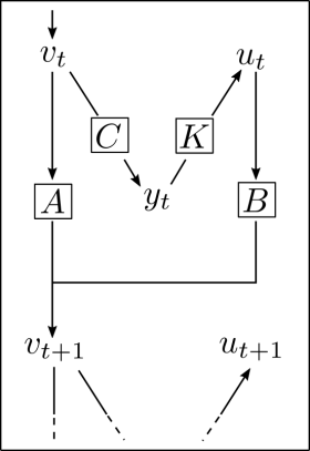
The above relationships are more compactly formulated mathematically as the linear system \((A, B, C)\):
\begin{align} \dot{v} & = Av(t) + B u(t), ~~~~~&&v\in \mathbb{R}^n, ~~ A\in \mathbb{R}^{n\times n}, ~~B\in \mathbb{R}^{n\times p} \\ y(t)&=Cv(t), && y\in \mathbb{R}^m, ~~ C \in \mathbb{R}^{m\times n} \end{align}
with matrices \(A, B, C\). It mediates between state vectors, control signals, and observations.
Controllability and observability
The system can be analyzed for controllability and the sufficiency of observations \(y\) for control using linear matrix inequalities. It is stated in [2] that:
- Either the system \((A,B,I)\) is controllable, or there exists a symmetric matrix \(P \neq 0\) such that $$ AP+PA^T \preceq 0, ~~PB=0.$$
Either the system \((A, B, C)\) is observable, or there exists a symmetric matrix \(P \neq 0\) such that $$ AP+PA^T \preceq 0, ~~C^TP=0.$$
From the solvability of semidefinite programs, global system properties can be derived.
Optimal control signals
For a system of the form \(\dot{x} = Ax + Bu\) with directly observable states \(x\), control signals can be directly derived from the state observations. The quadratic cost function \(\int_0^{\infty}u(t)^TRu(t)+x(t)^TQx(t) dt\) is to be minimized. This cost function consists of costs for the exertion of the control signal \(u(t)\) and costs for the deviation of the state \(x(t)\) from the desired stable state \(x=0\).
It follows that \(u = Kx\) with \(K\) being a matrix that maps states to control signals and satisfies the following matrix equations [3, pp. 35–40]:
\begin{align} K &= ‑R^{-1}B^TP \\ 0 &= A^TP + PA — PBR^{-1}B^TP + Q \\ P & \succeq 0 \end{align}
The equation for the matrix \(P\) is known as the algebraic Riccati equation and is quadratic in \(P\). The search for an \(K = ‑R^{-1}B^TP\) that optimally controls the system can be formulated as a semidefinite optimization problem in the matrix variable \(P\) [4, p. 9]:
$$ \begin{align} \min_P ~~~& -\operatorname{tr} P \\ \text{s.t.} ~~~&\begin{bmatrix} A^TP + PA + Q & PB \\ B^TP & R \end{bmatrix} \succeq 0 \\ ~~~& P \text{ symmetric} \end{align}$$
Applications
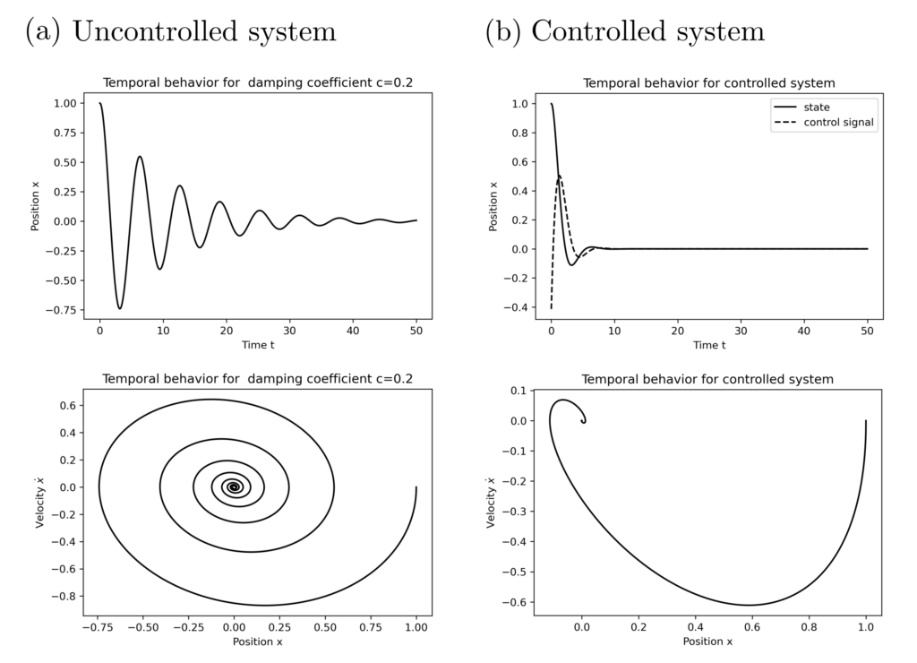
Given the damped harmonic oscillator now partially controllable with a control signal \(u\) according to the equation
\begin{align}
\dot{x} &= Ax + Bu \\
A &= \begin{bmatrix} 0 & 1 \\ ‑1 & ‑0.2 \end{bmatrix}, ~~~~~ B = \begin{bmatrix} 0 \\ 1 \end{bmatrix},
\end{align}
where \(x=[\text{Position, Velocity}]\). Then, under the constraints \(PB=0\) and \(A^TP+PA \preceq 0\) with \(P\) symmetric, it directly follows that \(\max (\operatorname{tr} P )=\min( \operatorname{tr} P)\) with the optimal \(P^*=0\) and the system is controllable. Simultaneously, \(PC^T=0\) and \(AP+PA^T \preceq 0\) with \(P\) symmetric and \(\max (\operatorname{tr} P )=\min( \operatorname{tr} P)\) with \(P^*=0\), and the system is observable. The solution of the semidefinite program
$$ \begin{align} \min_P ~~~& -\operatorname{tr} P \\ \text{s.t.} ~~~&\begin{bmatrix} A^TP+PA+I & PB \\ B^TP & 1\end{bmatrix} \succeq 0 \\ ~~~& P \text{ symmetric} \end{align}$$
is \(P^*=[1.73, 0.414; 0.414, 1.167]\) with \(K=-B^TP=[-0.414, — 1.167]\). With the control signal \(u^*=Kx\), the cost functional \(\int_{0}^{\infty} x^2(t)+\dot{x}(t)^2 + u^2(t) dt\) is minimized.
Practical aspects
If the matrices \(A\) and \(B\) are time-dependent, then the feedback matrix \(K\) is also time-dependent, and \(P\) satisfies a differential equation. If the relationships between \(x\), \(u\), and \(\dot{x}\) are nonlinear, optimal control might still be achievable. It should be investigated whether the effects of nonlinearity can be bounded by linear inequalities. The same considerations for nonlinearity also apply to random effects.
In practice, modeling a real-world phenomenon as a linear system \(\dot{x}=Ax+Bu\) is also challenging. This often requires higher-dimensional embeddings and linearizations, and despite all tricks, modeling might fail.
Due to the complexity of the real world, nonlinearity is a common complicating factor that softens guarantees of controllability and necessitates the introduction of experimental methods like reinforcement learning. Nonetheless, linear models and their analysis remain useful tools for investigating especially technical processes and those designed by humans.
Code & Sources
Example code: OC_harmonic_oscillator_1.py , OC_harmonic_oscillator_2.py in our tutorialfolder.
[1] Dym, C. L. (2002). Stability Theory and Its Applications to Structural Mechanics. New York: Dover Publications.
[2] Balakrishnan, V., & Vandenberghe, L. (2003). Semidefinite programming duality and linear time-invariant systems. IEEE Transactions on Automatic Control, 48,(1), 30–41.
[3] Anderson, B. D. O., & Moore, J. B. (2007). Optimal Control: Linear Quadratic Methods. New York: Courier Corporation.
[4] Yao, D. D., Zhang, S., & Zhou, X. Y. (2001). Stochastic Linear-Quadratic Control via Semidefinite programming. SIAM Journal on Control and Optimization, 40, (3), 801–823.
