Optimal control: Stochastic optimal control
Definition

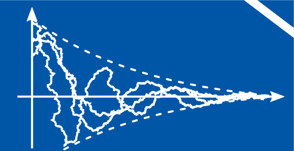
A system includes control inputs that can be chosen within certain limits and is to be stabilized through these inputs. The dynamics of the system, i.e., the influence of control input and current state on the future state, are known, but the system’s progression is still influenced by random disturbances.
This is an extension of optimal control with known dynamics and state to include random disturbances. The Linear-Quadratic Gaussian (LQG) control problem is an example of this problem class, where the disturbances are normally distributed.
LQG control
The dynamic model in the LQG can be written as
$$ x_{k+1} = Ax_k + Bu_k + w_k $$
with \(x_k, x_{k+1}\) typically being vector-valued states at times \(t=k, k+1\), \(u_k\) the control inputs, \(w_k\) the random disturbances, and \(A, B\) matrices. The control inputs are to be chosen such that stabilization of the system is achieved.
Given that the system dynamics matrices \(A, B\) are known, the variability of \(w\) quantifiable by the covariance matrix \(W\), and the control input \(u_k, k=1, … T \) is to be chosen such that the average energy is minimized. Formally, the optimization problem is
$$\min_{x_1, …, x_T, u_1, …, u_T} \lim_{T\rightarrow \infty} \frac{1}{T} E\left[ \sum_{k=0}^T \|x_k\|^2_Q + \|u_k\|^2_R\right] $$
where \(\|x_k\|^2_Q=x_k^TQx_k\) and \(\|u_k\|^2_R=u_k^TRu_k\) are measures for the costs of state \(x_k\) and control input \(u_k\), and \(E[\cdot]\) is the expectation value.
SDP Formulation
The optimal control input \(u_k\) is determined by the equation [1] \(u_k=Z_{xu}^T(Z_{xx})^{-1} x_k\) where \(Z_{xx}\) and \(Z_{xu}\) are solutions to the following semidefinite program [2].
$$\begin{align} \min_{Z_{xx}, Z_{xu}, Z_{uu}} ~~~&\operatorname{tr} (QZ_{xx}) + \operatorname{tr} (R Z_{uu}) \\ s.t. ~~~& \begin{bmatrix} Z_{xx} & Z_{xu} \\ Z_{xu}^T & Z_{uu} \end{bmatrix} \succeq 0 \\ & Z_{xx}-AZ_{xx}A^T‑AZ_{xu}B^T — BZ_{xu}^TA^T — B Z_{uu}B^T=W\end{align}$$
The function to be minimized, \(\operatorname{tr} (QZ_{xx}) + \operatorname{tr} (R Z_{uu})\), quantifies expected costs (money, time, energy, errors) through the relationship $$E[X^TQx+u^TRu]=\operatorname{tr}(Q E[xx^T])+\operatorname{tr}(RE[uu^T])=\operatorname{tr}(QZ_{xx})+\operatorname{tr}(RZ_{uu}).$$ Thus, \(Z_{xx}\) and \(Z_{uu}\) can be interpreted as covariance matrices of the randomly distributed variables \(x\) and \(u\), and the equation \(u_k=Z_{xu}^T(Z_{xx})^{-1}x_k\) is precisely the conditional expectation of \(u_k\) given \(x_k\) and the probability distribution determined by \(Z_{xx}, Z_{xu}, Z_{uu}\) that minimizes energy.
Example: Pendulum control
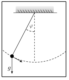
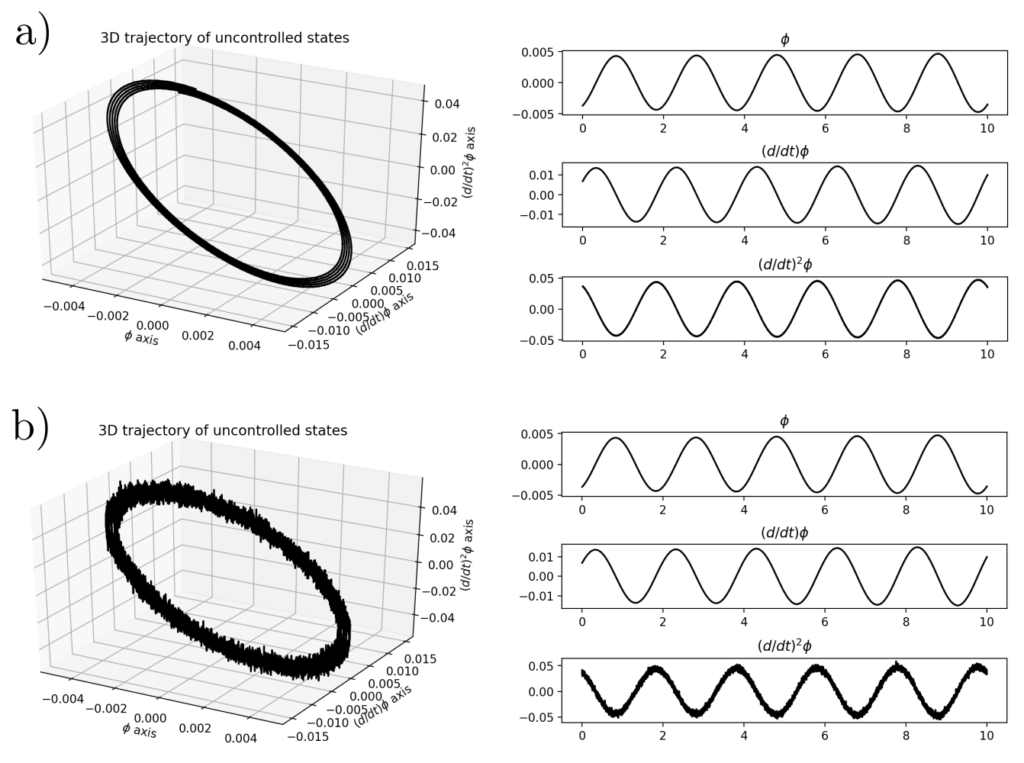
In the following detailed example, the objective is to stabilize a pendulum affected by random effects. We assume that a pendulum starts from a random (but small) deviation \(\varphi\) from the equilibrium position.
The pendulum motion then follows normal physical laws, with the exception that additional random effects, neither predictable nor controllable by us, cause a force and thus an acceleration on the pendulum.


Note that the graph shows the expected behavior for pendulum oscillations. When the displacement \(\varphi\) is maximal, then the velocity \(\dot{\varphi}=0\) and the acceleration \(\ddot{\varphi}\) is minimal. When the displacement \(\varphi=0\), the velocity \(\dot{\varphi}\) is maximal, and the acceleration \(\ddot{\varphi}\) switches from positive to negative or vice versa.
Pendulum equations
The acceleration induced by the gravitational force \(g\) in the direction of oscillation is \(-g\sin(\varphi)\). Furthermore, random effects \(w\) are acting, and we assume that the control input \(u\) we choose directly affects the acceleration, such that
$$\ddot{\varphi}_k = ‑g \sin(\varphi_k) + w_k + u_k ~~~~~~~k=0, …, T.$$
The state equation coupling different quantities over successive time steps can be written as
$$ \underbrace{\begin{bmatrix} \varphi_{k+1} \\ \dot{\varphi}_{k+1} \\ \ddot{\varphi}_{k+1} \\ \sin(\varphi_{k+1}) \\ \cos(\varphi_{k+1}) \end{bmatrix}}_{x_{k+1}} = \underbrace{\begin{bmatrix} 1 & \Delta t & 0 & 0& 0 \\ 0 & 1 & \Delta t & 0 & 0 \\ 0& 0& 0& ‑g & 0 \\ 0 & \Delta t & 0 & 1 & 0 \\ 0&0&0&0&0\end{bmatrix}}_{A}\underbrace{\begin{bmatrix} \varphi_{k} \\ \dot{\varphi}_{k} \\
\ddot{\varphi}_{k} \\ \sin(\varphi_{k}) \\ \cos(\varphi_{k})
\end{bmatrix}}_{x_{k}} + \underbrace{\begin{bmatrix} 0 \\ 0\\ 1 \\ 0\\0 \end{bmatrix}}_{B} \underbrace{\begin{bmatrix} u_k\end{bmatrix}}_{u_k} + \underbrace{\begin{bmatrix} 0\\0\\w_k\\0\\0 \end{bmatrix}}_{w_k}.$$
The approximations valid for small angles
$$\begin{align} \sin (\varphi+\Delta \varphi)&\approx \sin\varphi+\Delta \varphi \cos \varphi\approx \sin \varphi + \Delta t \dot{\varphi} \cos \varphi \approx \sin \varphi + \Delta t \dot{\varphi} \\ \cos(\varphi+\Delta\varphi) &\approx \cos \varphi — \Delta \varphi \sin \varphi \approx \cos \varphi — \Delta t \dot{\varphi} \sin \varphi \approx \cos \varphi \end{align}$$
are used to create the last two rows of the equation.
Solution
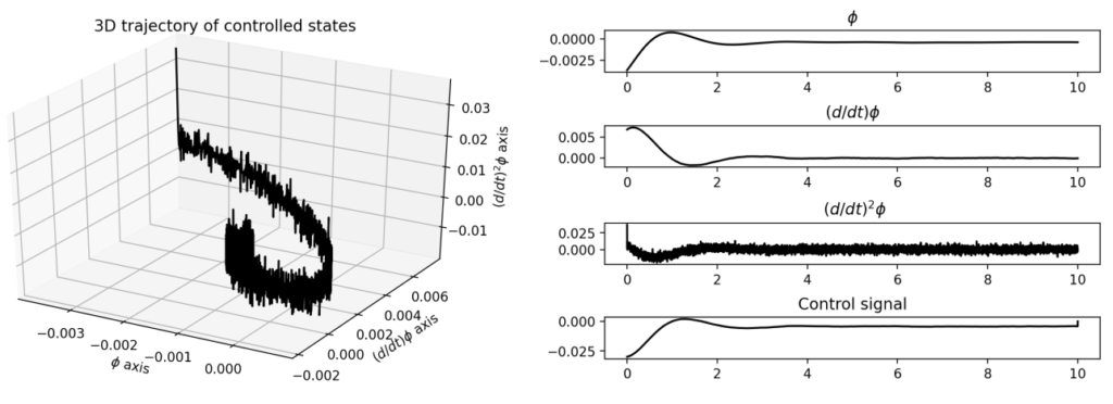
To find a matrix \(K\) such that the control input \(u_k=Kx_k\) stabilizes the system, the optimization problem
$$\begin{align} \min_{Z_{xx}, Z_{xu}, Z_{uu}} ~~~& \sum_{i=1}^3 (Z_{xx})_{ii} +(Z_{uu})_{ii} \\ s.t. ~~~& \begin{bmatrix} Z_{xx} & Z_{xu} \\ Z_{xu}^T & Z_{uu} \end{bmatrix} \succeq 0 \\ & Z_{xx}-AZ_{xx}A^T‑AZ_{xu}B^T — BZ_{xu}^TA^T — B Z_{uu}B^T=W\end{align}$$
needs to be solved. Here, \(A\) and \(B\) are as described in the previous section, \(w\) is a \(5 \times 5\) matrix of \(0\)s except for the entry \(W_{33}=\sigma_w^2\) representing the variance of the random effect on acceleration, and the resulting control signal is \(u_k= Kx_k=Z_{xu}^T(Z_{xx})^{-1}x_k\).

Practical aspects
To adapt the above solution approach to other systems, several considerations must be kept in mind. The system dynamics must be linear, thus formulable as $$x_{k+1}=Ax_k+Bu_k+w_k$$ where the \(w_k\) must be independent random variables with a known covariance matrix. If the \(w_k\) are correlated with each other, the entire optimization equation must be embedded into a higher-dimensional space that incorporates both \(x_1, …, x_k\) and \(w_1, …, w_k\) simultaneously.
Even in the pendulum example, the state \(x_k\) was 5‑dimensional with two auxiliary dimensions documenting \(\sin \varphi_k\) and \(\cos \varphi_k\). The definition of the state vector must be conducted by the user themselves and can become quite complicated. Often, tricks and approximations are necessary to transform nonlinear equations into a linearized form that is usefully applicable.
Code & Sources
Example code: OC_stochastic_control_1.py , OC_stochastic_control_2.py in our tutorialfolder.
[1] Balakrishnan, V., & Vandenberghe, L. (2003). Semidefinite programming duality and linear time-invariant systems. IEEE Transactions on Automatic Control, 48,(1), 30–41.
[2] Kamgarpour, M., Summers, T. (2017). On infinite dimensional linear programming approach to stochastic control. 20th IFAC World Congress (IFAC 2017), Toulouse, France, July 9–14. IFAC-PapersOnLine, 50, (1), 6148 — 6153.
