Optimal design: Transportation and resource flow
Definition

When resources need to be distributed across various locations, and distribution is only possible along certain routes, the resulting problem is called a routing problem. This encompasses the design of optimal flows of goods, energy, or information through complex networks.
These are problems that particularly arise in the transportation sector, where they manifest as questions about the shortest routes for goods transportation. According to studies such as [1], up to 13% of a product’s total manufacturing costs can be attributed to transportation costs, presenting significant opportunities for savings.
Origin: Route design
The so-called Travelling Salesperson Problem (TSP) is an archetypal routing problem that was mathematically formulated in the 19th century. In the TSP, a salesperson needs to visit a set of locations and choose the sequence of sites such that the total duration of the tour is minimized.
The problem seems trivial but is proven to be one of the most difficult mathematical challenges. Furthermore, its relevance extends far beyond transportation. Data clustering, wiring of microchips, arranging semiconductor components into an integrated circuit, airport design, and controlling large telescopes to target multiple celestial bodies can all be formulated in the language of routing planning. See, for example, [2].
TSP: Example
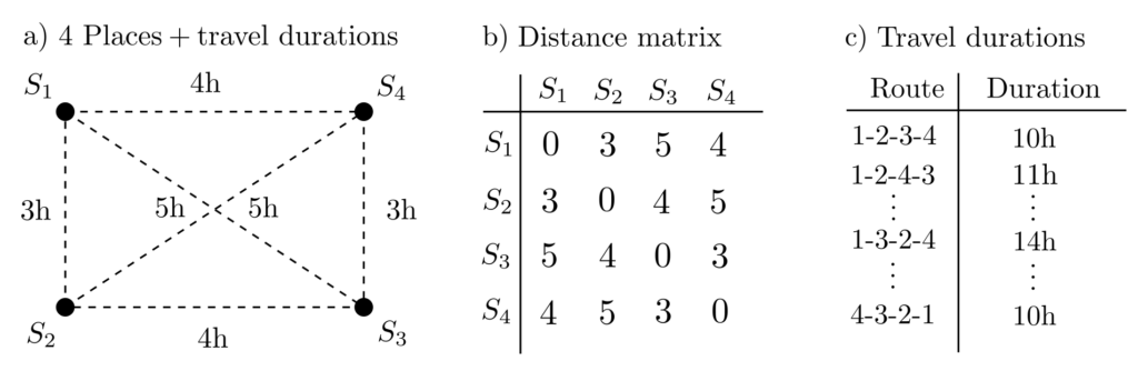
The TSP is a prototype for many transportation and resource flow problems. Even an instance with just a few locations to visit highlights the difficulties. Suppose there are 4 locations to be visited in such a way that the travel time is minimized. For simplicity, we omit the constraint that the starting point and endpoint should be identical.

The shortest tour in the above example is \(1\rightarrow 2\rightarrow 3\rightarrow 4\) with a travel time of 10 hours. However, this result is only apparent after all \(4! = 4*3*2*1 = 24\) possible tours have been calculated and their lengths compared. This method, based on reviewing all possible options, rapidly loses practicability with an increasing number of destinations. For 12 locations, already 500,000,000 options must be calculated. The introduction of constraints and more complex objective functions requires a completely different approach to solving the problem.
Optimization formulation
Routing problems like the TSP can be formulated using mixed-integer linear optimization. To do this, binary variables \(x_{ij} \in \{0,1\}\) are introduced, which indicate whether the direct route from point \(i\) to point \(j\) is taken or not. With \(c_{ij}\) representing the travel times between points \(i\) and \(j\), the optimization problem is as follows [3]:
$$\begin{align}
\min{x_{ij}} ~~~ & \sum_{i=1}^n \sum_{j=1, j\neq i}^n c_{ij}x_{ij} &&\\
\text{s.t.} ~~~& \sum_{i=1, i \neq j}^n x_{ij}=1 &&j=1, …, n \\
&\sum_{j=1, j\neq i}^n x_{ij}=1 && j=1, …, n \\
& \sum_{i \in Q} \sum_{j\in Q, j\neq i} x_{ij}\le |Q|-1 && \forall Q\underset{\neq}{\subset} \{1, … , n\}, |Q|\ge 2
\end{align}$$
The role of the constraints is to enforce a flow on the transport network where each location is visited and left exactly once and which contains no loops.
Generalization
To address the complexity of real-world problems, practice shows that additional constraints and model details are necessary. For example, the following situations need to be modeled:
- The presence of multiple transport vehicles and the possibility to rent additional ones
- Capacity limitations of delivery vehicles
- Maximum permissible driving durations and fixed time frames for deliveries
- Simultaneous deliveries and product returns
- Penalties for undelivered shipments
- Random effects and robust tour plans
All of this makes tour planning problems often have very complicated mathematical formulations with a daunting amount of equations.
Example
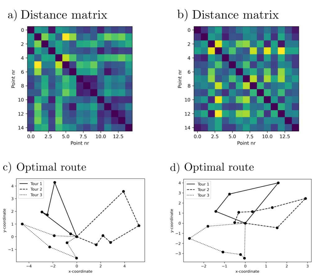
Three vehicles are available to travel through a set of \(n=45\) locations \(v_i, i=1, \ldots, n\), in such a way that the length of the longest tour is minimized. This can be formulated as the optimization problem [4, p. 154]:
$$\begin{align} \min_{x_{ij}} ~~~& \max\left(\sum_{i<j} c_{ij}x_{ij}^1, \sum_{i<j}c_{ij}x_{ij}^2, \sum_{i<j} c_{ij}x_{ij}^3\right) \\ \text{s.t.} ~~~& x(\delta(\{v_0\}))=6 && \\ &x(\delta(\{v_i\}))=2 && i=1, \ldots, n \\ & x(\delta(S)) = 6 && S\subseteq V\setminus\{v_0\} \\ & 0 \le x_{0j}^k \le 2 && j=1, \ldots, n,~~~ k=1, 2, 3 \\ & 0 \le x_{ij}^k \le 1 && i < j,~~~ i,j =1, \ldots, n,~~~ k=1, 2, 3 \\ & x_{ij}^k \in \mathbb{Z} && i\le j, ~~~ i,j=1, \ldots, n, ~~~ k=1, 2, 3 \end{align}$$
Here, \(x_{ij}^k\) is an indicator variable that denotes whether vehicle \(k\) travels from \(i\) to \(j\), \(V=\{v_0, \ldots, v_n\}\) represents the set of all locations including the start and endpoint \(v_0\), and \(\delta(S)\) is the set of connections leading out of the set \(S\). The term \(x(\delta(S))\) represents the sum of the actual connections leading out of the set \(S\).

Solution
Note that the requirement \(x(\delta(S))=6 \forall S \subseteq V \setminus \{v_0\}\) includes an equation for each subset of \(V=\{v_1, …, v_n\}\). Since there are exponentially many equations, these equations are typically neither manually formulable nor solvable and are also not accessible to a normal computer. E.g. if the number of locations in the above example are increased to 30, the amount of equations from that constraint alone number at least \(2^{30}\approx 1\) billion.
However, powerful software exists that can approximately solve these problems using heuristics. For the above example, we used the OR-Tools library from Google—a toolbox with a Python interface that specifically deals with providing algorithms for operations research. More information about the package, which was significantly developed by Laurent Perron and Vincent Furnon and is publicly available, can be found here .
Practical aspects
Due to the difficulty of exactly solving tour planning problems, algorithms have been developed that quickly lead to good, though probably not optimal, tours. Given the economic significance of transport problems, a lot of work has gone into developing various heuristics, and some practical rules have emerged that can be used ad hoc by users without significant computational effort.
An example of this is the largest-gap strategy, by which forklift operators choose their routes in a warehouse [5]. Tour planning problems, therefore, are still not exactly solvable but at least approximately so. And the routes found through optimization are often 10–15% better than those planned manually [4, p. 153].
Code & Sources
Example code: OD_routing.py in our tutorialfolder
[1] Owoc, M., & Sargious, M. A. (1992). The Role of Transportation in Free Trade Competition. In N. Waters (ed.), Canadian Transportation: Competing in a Global Context. Banff, Alberta, Canada.
[2] Lenstra, J. K. & Rinnooy, K. (1975). Some Simple Applications of the Travelling Salesman Problem. Operational Research Quarterly, 26(4), 717–733.
[3] Dantzig, G., Fulkerson, R., & Johnson, S. (1954). Solution of a large-scale Travelling Salesman Problem. Journal of the Operations Research Society of America, 2(4), 393–410.
[4] Appa, G. M., Pitsoulis, L., & Williams, H. P. (2006). Handbook on Modelling for Discrete Optimization. Berlin, Heidelberg: Springer.
[5] Petersen, C. G. (1997). An Evaluation of Order Picking Routing Policies. International Journal of Operations & Production Management, 17, 1096–1111.
