Optimal control: Planning problems
Problem setting

A system receives control inputs that can be chosen freely within certain limits and is supposed to be brought into a predefined state or follow a specific trajectory. However, in this complete generality, the problem is difficult to manage.
Complicating factors such as nonlinearities, unknown system dynamics, and randomness in the interactions between control input and system response can make the problem completely unsolvable.
In the simplest case of complete predictability of the system, however, it is a static planning problem, and a solution can be reduced to the search for a sequence of control inputs. This search can be conducted with the help of dedicated search algorithms such as the Monte-Carlo Tree Search, or it can be formulated as an optimization problem in which the system dynamics take on the role of constraints.
Mathematical model
If the state \(x_{k+1}\) at time \(k+1\) depends linearly on the previous state \(x_k\) and the control input \(u_k\), the system dynamics can be written as
$$x_{k+1}=Ax_k+Bu_k $$
where \(x_{k+1}, x_k \in \mathbb{R}^d, u_k\in \mathbb{R}^m\) are typically multidimensional vectors. \(A\) and \(B\) are system matrices that encode the influence of the state and control signal on the future state. If the system is to be controlled such that it follows a trajectory \(f_1, …, f_n \in \mathbb{R}^d\) with as small a control input as possible, this can be formulated as the optimization problem
$$ \begin{align} \min_{x_1, …, x_n, u_1, …, u_n} ~~~& \sum_{k=1}^n \|x_k-f_k\|_1+\|u_k\| \\ \text{s.t.} ~~~&x_{k+1}=Ax_k+Bu_k~~~ k=1, …, n \\ ~~~& x_1=x_{start} \end{align}$$
where \(x_1\) is set as the starting state \(x_{start}\). The optimization variables are the \(n\) control inputs \(u_1, …, u_n\) and the states \(x_1, …, x_n\), constrained by the dynamic constraints. It is an optimization problem with \(nd+nm\) variables.
It can be reformulated as a linear program with the objective function \(\|x‑f\|_1+\|u\|_1=\|v^{\Delta}\|_1+\|v^u\|_1\) where \(x=[x_1^T, …, x_n^T]^T\) and \(u=[u_1^T, …, u_n^T]^T\) with \(v^{\Delta} \in \mathbb{R}^{nd}\) and \(v^u\in \mathbb{R}^{nm}\) being the vectors of the absolute values of the elements of \(x‑f\) and \(u\).
$$ \begin{align} \min_{x_1, …, x_n, u_1, …, u_n, v^{\Delta}, v^u} ~~~& \sum_{k=1}^n\sum_{l=1}^d v^{\Delta}_{kl}+ \sum_{k=1}^n \sum_{l=1}^m v^u_{kl} \\ \text{s.t.} ~~~&x_{k+1}=Ax_k+Bu_k~~~ k=1, …, n \\ ~~~& v^{\Delta} \ge x‑f ~~~ v^{\Delta}\ge -(x‑f) \\ ~~~& v^u\ge u ~~~~~~~~~~~ v^u \ge ‑u \end{align}$$
The first inequality represents the dynamics of the system while the last two pairs ensure the positivity of the absolute residuals \(v^{\Delta}\) and \(v^u\) [1, p. 294].
Example: Motion control
A drone is to be controlled so that it moves from its current 3‑dimensional position \(pos_1=[x_{start}, y_{start}, z_{start}]\) to the target position \(pos_n=[x_{Ziel}, y_{Ziel}, z_{Ziel}]\) within \(n\) time steps, arriving with a velocity of \(v_n=[v^x_{Ziel}, v^y_{Ziel}, v^z_{Ziel}]\). The control signal \(u\), which should be kept as small as possible, is directly translated into acceleration, so that the relationship
$$x_{k+1}= \begin{bmatrix} pos_{k+1} \\ v_{k+1} \\ a_{k+1}\end{bmatrix} = \underbrace{\begin{bmatrix} I & \Delta t I & 0 \\ 0 & I & \Delta tI \\ 0 & 0 & \Delta t I\end{bmatrix}}_{A} \underbrace{\begin{bmatrix} pos_k \\ v_k \\ a_k\end{bmatrix}}_{x_k}+\underbrace{\begin{bmatrix} 0 \\ 0 \\ \Delta t I \end{bmatrix}}_{B} \underbrace{\begin{bmatrix}u_x \\ u_y\\ u_z\end{bmatrix}}_{u_k}$$
is valid. Here, \(I\) is the \(3 \times 3\) identity matrix, \(\Delta t\) is the duration of one time step, \(pos\) stands for position, \(v\) for velocities, and \(a\) for accelerations. Each state vector thus has 9 components.

Solution and practical aspects
The corresponding optimization problem is
$$ \begin{align} \min_{x_1, …, x_n, u_1, …, u_n}
~~~& \sum_{k=1}^n\|u_k\|_1 \\ \text{s.t.} ~~~&x_{k+1}=Ax_k+Bu_k~~~ k=1,
…, n \\ ~~~& pos_1=[x_{Start}, y_{Start}, z_{Start}]^T ~~~~pos_n=[x_{Ziel}, y_{Ziel}, z_{Ziel}]^T \\~~~& v_1=[v^x_{Start}, v^y_{Start}, v^z_{Start}]^T ~~~~~~~~~~~~v_n=[v^x_{Ziel}, v^y_{Ziel}, v^z_{Ziel}]^T\\ ~~~& u_{min}\le u_k \le u_{max} ~~~k=1, …,n .\end{align}$$
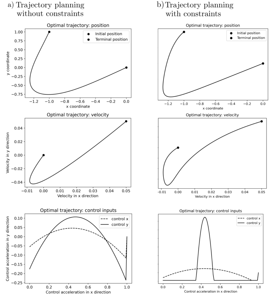
An illustration of the problem is located in the following figure. Note that the final control inputs and trajectory significantly depend on the starting conditions and possible control input restrictions.

The problem is solved using the freely available software CVXOPT [2] and CVXPY [3] on a standard laptop within a few milliseconds. There are various extensions. The objective function typically contains quadratic terms, and it is possible to model uncertainties in system dynamics and the environment through random variables. This leads to the Linear-Quadratic Gaussian (LQG) controllers [4, pp. 164–207]. To avoid complex optimizations, it is often required that \(u\) be directly representable as a function of \(x\) with \(u=Kx\) and a constant matrix \(K\); see, for example, [5, pp. 421–441].
Code & Sources
Examplecode: OC_vehicle_control_3.py in our tutorialfolder.
[1] Boyd, S., & Vandenberghe, L. (2004). Convex Optimization. Cambridge: Cambridge University Press.
[2] Andersen, M. S., , Dahl, J., & Vandenberghe, L. (2022) . CVXOPT: A Python package for convex optimization, version 1.3
[3] Diamond S., & Boyd S., (2016). CVXPY: A Python-embedded modeling language for convex optimization. Journal of Machine Learning Research, 17(83), 1–5.
[4] Anderson, B. D. O., & Moore, J. B. (2007). Optimal Control: Linear Quadratic Methods. New York: Courier Corporation.
[5] Wolkowicz, H., Saigal, R., & Vandenberghe, L. (2012). Handbook of Semidefinite Programming: Theory, Algorithms, and Applications. Berlin Heidelberg: Springer Science & Business Media.
