Optimal control: Reinforcement learning
Definition
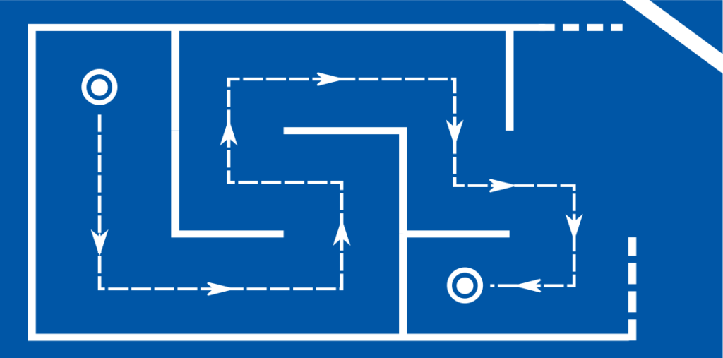
Reinforcement learning (RL) is a method for optimal control under very challenging conditions. The state changes are random, the probabilities are unknown, and the function to be optimized itself has no closed form. Despite these challenges, an optimal policy is to be found.
A policy is understood to be a plan that specifies for every possible state the control signal that leads to the best results in the long run. The range of tasks that can be formulated in this way is so general that everything from machine control, adaptive planning of search-and-rescue missions, to the development of independently learning chess algorithms that play at a world champion level can be considered an RL problem.
Example
An example of an optimal control problem that can be instructively solved with RL is the navigation of a maze from the starting point \(A\) to the target point \(B\). The layout of the maze is unknown but locally queryable by the algorithm navigating the maze. Since the algorithm can actively interact with its environment to gain information, it is also referred to as an agent. Describing the above problem as an LP, QP, … SDP would be — if at all possible — enormously difficult.

Exemplary analysis
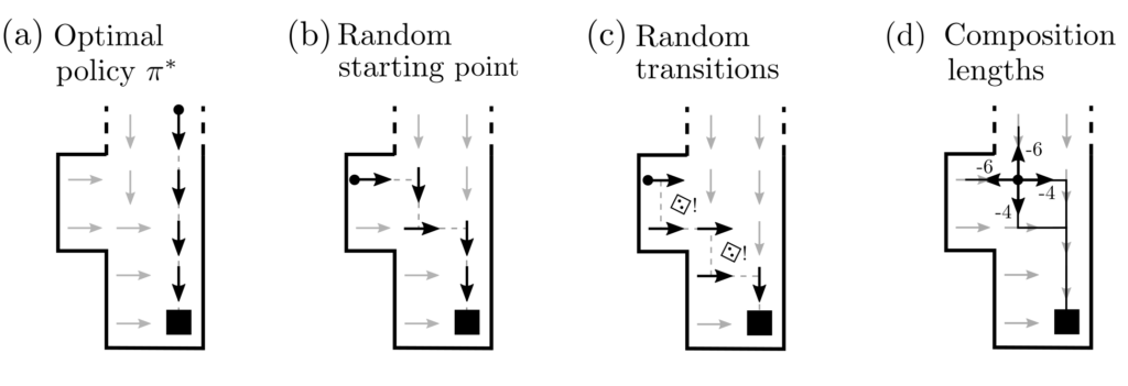
The solution to the maze problem is a policy \(\pi^*:S \ni s \mapsto \pi^*(s) \in A\), which accepts a position \(s \in S\) as input and generates an action \(a \in A\) as output. This solution proposes not just a rigid plan of positions \(s_A, s_1, …, s_B\), but solves the planning problem for all possible starting positions simultaneously. If the agent were now placed at any position \(s_0\) and is to find the shortest way to \(B\) from there, it would succeed by following the policy
$$s_0\stackrel{\pi^*(s_0)=a_0}{\rightarrow} s_1\stackrel{\pi^*(s_1)=a_1}{\rightarrow} …\stackrel{\pi^*(s_n)=a_n}{\rightarrow}s_B .$$
The same applies if the position changes are influenced by chance and the exact subsequent position does not follow 100% from the past positions and the chosen action.
Formulation of RL tasks
RL problems are formalized similarly to Markov decision processes. As input for RL algorithms, a computer model is needed that:
- Defines the state space \(S\) and the action space \(A\)
- Generates a (stochastic) reward \(r(s,a)\) for each pair \((s,a)\in S\times A\)
- Generates a (stochastic) successor state \(s’(s,a)\) for each pair \((s,a)\in S \times A\).
These requirements are somewhat weaker and practically easier to manage than for Markov decision processes. Instead of a tabular, comprehensive capture of the rewards \(r(s,a)\) and transition probabilities \(p(s’|s,a)\) between states, RL merely requires examples. The goal is to determine an optimal policy \(\pi^*\), which maximizes the expected value of cumulative rewards.
$$ \begin{align} \max_{\pi} ~~~&E_{\pi}\left[ \sum_{k=1}^{\text{End}} r(s_k,a_k)\right] \\ \text{s.t.} & a_k=\pi(s_k)\end{align}$$
Here, \(E_{\pi} \left[\sum_{k=1}^{\text{End}}r(s_k,a_k)\right]=\eta(\pi)\) denotes the expected value of cumulative rewards when the policy \(\pi\) is followed.
Solution
There are various approaches to determining \(\pi^*\). What they have in common is that the agent collects data through interaction with the computer model, and the experiences about states, actions, state changes, and rewards are fed into a feedback loop to determine \(\pi^*\).
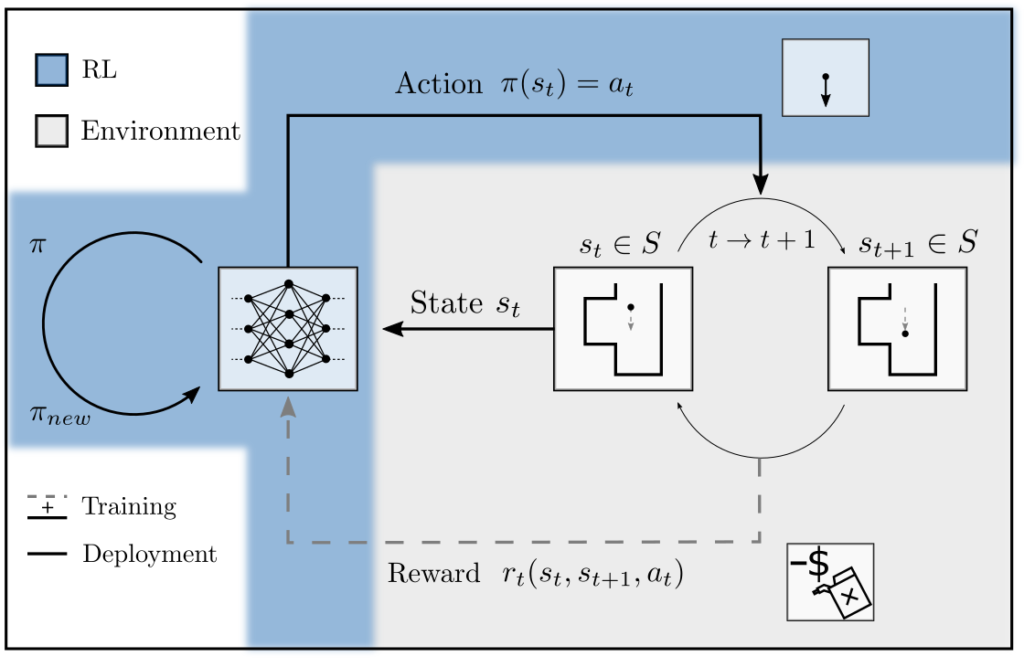
The function \(\pi:A\rightarrow S\) is often constructed as a neural network \(\pi_{\theta}\) for reasons of flexibility. It can then be adjusted based on the data by, for example, forming the derivatives of \(\eta(\pi)\) with respect to the parameters \(\theta\) of \(\pi\) [1, p. 367].
$$\begin{align} \eta(\pi) & =\int_{(S\times A)^n} \sum_{k=0}^nr(s_k,a_k)p_{\theta}(\xi)d\xi \\ \nabla_{\theta} \eta &= \int_{(S\times A)^n}\sum_{k=0}^n r(s_k,a_k) \nabla_{\theta}\left[ \log p_{\theta}(\xi)\right] p_{\theta}(\xi)d\xi \\ \hat{\nabla}_{\theta} \eta & = \frac{1}{m}\sum_{j=1}^m \left( \sum_{k=0}^n r(s_k^j,a_k^j)\right)\nabla_{\theta}\left[ \log p_{\theta}(\xi)\right] \\ & =\frac{1}{m} \sum_{j=1}^m \left( \sum_{k=0}^n r(s_k^j,a_k^j)\right)\sum_{k=0}^n\nabla_{\theta}\log \pi_{\theta}(s_k^j,a_k^j)\end{align}$$
Here, \(p_{\theta}(\xi)\) is the probability of occurrence of the sequence \([(s_0,a_0), …, (s_n,a_n)]\), and \(\hat{\nabla}_{\theta} \eta\) is a data-driven estimator for the gradient of cumulative reward. The above equations are used, for example, in the TD3 algorithm [2] and are implemented in the Python library Stable Baselines3 [3].
Example: Landing control
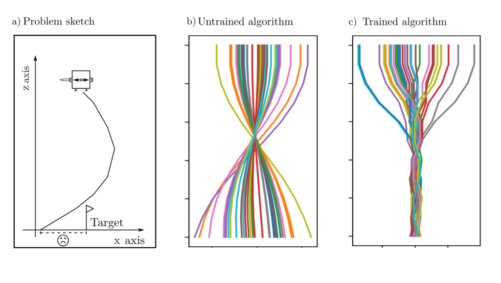
The landing process of an object is to be controlled so that it lands at the designated coordinate \(0\). The landing process follows the usual differential equations that couple position, velocity, and acceleration, but this is not known to the algorithm. Upon touching the ground after time \(T\), a reward of \(-|x(T)|\) is dispensed, which penalizes the deviation from the actual and designated landing point, thus defining it as something to be minimized.
Example: Adaptive control of measurement density
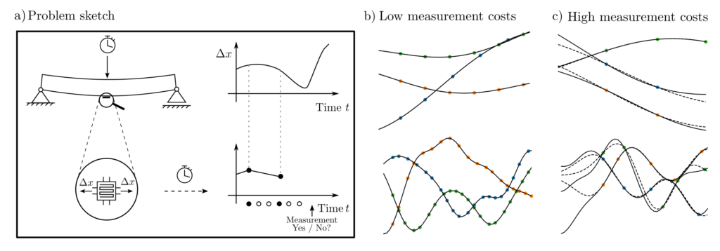
A sensor is to measure the temporal motion behavior of an object in such a way that it can be reconstructed as accurately as possible. However, each measurement costs money; therefore, the measurement times must be chosen economically. The computer model of this problem includes randomly generated functions, the option for a motion measurement at any point in time, and at the end of the trial run, a consideration of measurement costs and reconstruction error as a performance measure.
Example: Adaptive search policy
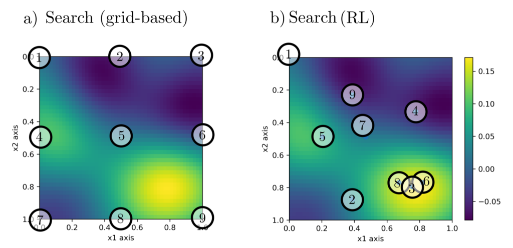
On a property contaminated with pollutants, the location and severity of the maximum contamination are to be determined. To do this, 9 pollutant measurements can be conducted at freely chosen locations, and the algorithm should adaptively decide on the location of the next measurement based on previous measurements. The training data consist of simulations that are presumed to have a correlation structure similar to the pollutant distribution in the real world.
Practical aspects
Reinforcement learning can be used for almost anything, including problems of high-dimensional nature with high demands on the algorithm’s learning ability. However, this flexibility also entails significant disadvantages. RL is enormously data-hungry, has stability issues, and places high modeling requirements on the user. The user must design state and action spaces in such a way that the dynamics have Markov properties and must balance flexibility and regularity through the architecture of the involved artificial neural networks.
If a problem can be formulated as an established convex optimization task, RL should be avoided. For many other problems, despite its pitfalls, RL is the only viable approach. Since it is a method that is still actively and intensively researched, significant advances can be expected in the future.
Code & Sources
Example code: OC_RL_class_def_2D_env-py , OC_RL_def_2D.py , OE_RL_control_trajectory.py , OC_RL_measurement_decisions.py , OC_RL_support_funs.py , OC_RL_trained_benchmark_def_2D.zip in our tutorialfolder.
[1] Wiering, M., & Otterlo, M. v. (2012). Reinforcement Learning: State-of-the-Art. Berlin Heidelberg: Springer Science & Business Media.
[2] Fujimoto, S., van Hoof, H., & Meger, D. (2018). Addressing function approximation error in actor-critic methods. arXiv preprint arXiv:1802.09477, 2018.
[3] Raffin, A., Hill, A., Gleave, A., Kanervisto, A., Ernestus, M., & Dorman, N. (2021). Stable-Baselines3: Reliable Reinforcement Learning Implementations. Journal of Machine Learning Research. 22, (268), 1−8.
