Optimal design: Experiment design
Problem statement

The question of the optimal design of an experiment or a measurement setup arises wherever the collection of measurements is costly and fraught with uncertainties. This concerns any applications where data analysis must be performed using statistical methods.
This includes the design of pharmaceutical trial series [1, p. 511], school exams [2], or measurement networks in geodesy [3]. In experimental design, the goal is to determine how often and which measurements should be conducted to maximize the information content of the data.
Example: Measurement distribution
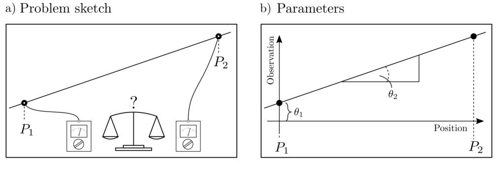
A line is to be drawn through data points measured at two positions. This task alone would be a trivial one from the field of parameter estimation. However, we are now dealing with the question of how a measurement budget of, for example, \(N=10\) noisy measurements can be allocated to these positions in such a way that the overall uncertainty of the estimated line is minimized. This is precisely an experiment design problem.

The relationship between measurements \(l_1\), \(l_2\) and positions \(p_1, p_2\) is given by the equation of a line as
$$ \underbrace{\begin{bmatrix} l_1 \\ l_2 \end{bmatrix}}_{l} \approx \underbrace{\begin{bmatrix} 1 & p_1 \\ 1 & p_2 \end{bmatrix}}_{A} \underbrace{\begin{bmatrix} \theta_1 \\ \theta_2 \end{bmatrix}}_{\theta} ~~~~~\begin{matrix} \theta_1 : \text{ Intercept} \\ \theta_2 : \text{ Slope} \end{matrix}.$$
\(n_1\) measurements can be taken at \(p_1\) and \(n_2\) measurements at \(p_2\), where \(n_1 + n_2 = N = 10\) must hold.
Example: Optimization formulation
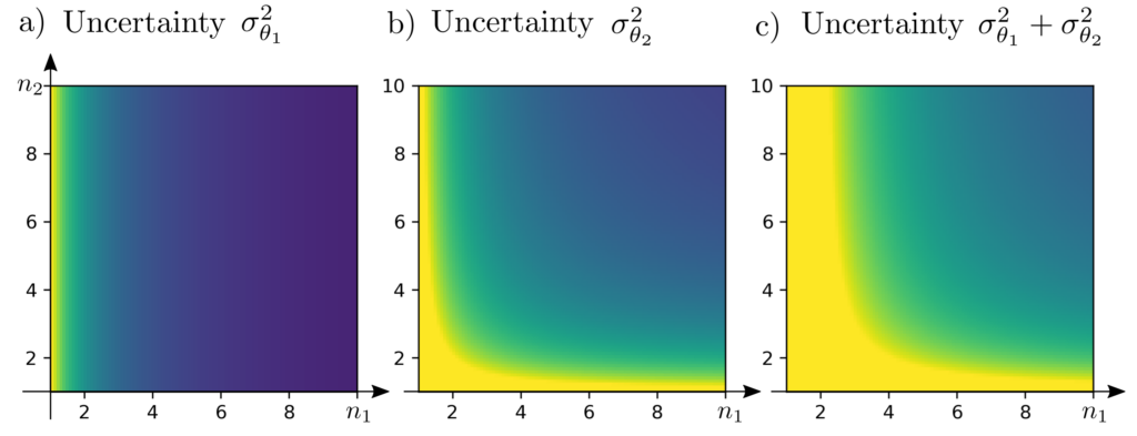
This measurement distribution is to be chosen such that the total uncertainty \(\sigma_{\theta_1}^2 + \sigma_{\theta_2}^2\) of the parameters is minimized, where \(\sigma_{\theta}^2\) is the variance of the parameter \(\theta\). The optimization problem is
$$\begin{align} \min_{n_1,n_2} ~~~ & \sigma_{\theta_1}^2(n_1,n_2) + \sigma_{\theta_2}^2 (n_1, n_2) \\ \text{s.t.} ~~~ & n_1+n_2=10 \end{align}$$
For simplicity, let’s assume that the measurements are equally accurate with variance \(\sigma_0^2\) and choose the specific measurement positions \(p_1=0\) and \(p_2=1\). According to the usual rules for uncertainties, an \(n-\) fold measurement reduces the variance to \(1/n-\) of the single measurement variance [4, p. 17]. Then, for the covariance matrices \(\Sigma_l, \Sigma_{\theta}\) of the observations and the parameters,
$$\begin{align} \Sigma_l & = \sigma_0^2 \begin{bmatrix} \frac{1}{n_1} & 0 \\ 0 & \frac{1}{n_2} \end{bmatrix} \\ \Sigma_{\theta} & =A^{-1} \Sigma_l A^{-1 T} \\ & = \sigma_0^2 \begin{bmatrix} 1 & 0 \\ ‑1 &1 \end{bmatrix} \begin{bmatrix} \frac{1}{n_1} & 0 \\ 0 & \frac{1}{n_2} \end{bmatrix} \begin{bmatrix} 1 & ‑1 \\ 0 & 1 \end{bmatrix} \\ & = \sigma_0^2 \begin{bmatrix} \frac{1}{n_1} & — \frac{1}{n_1} \\ -\frac{1}{n_1} & \frac{1}{n_1}+\frac{1}{n_2} \end{bmatrix} \end{align} $$
Minimizing \(\sigma_{\theta_1}^2 + \sigma_{\theta_2}^2\) is equivalent to minimizing \(\operatorname{tr} \Sigma_{\theta} \) and thus, the optimal experimental design is characterized by
$$\begin{align} \min_{n_1,n_2} ~~~& \frac{2}{n_1}+\frac{1}{n_2} \\ \text{s.t.} ~~~ & n_1+n_2=10 \end{align}$$
Example: Solution
Surprisingly, the measurement at location \(p_1\) is twice as important for the overall uncertainty as the measurement at location \(p_2\). This is because the measurement \(l_2\) is irrelevant for the parameter \(\theta_1\) — a relationship that would not have been considered in an intuitive equal distribution of measurements.
The constrained optimization problem can be solved using the Lagrange function \(\mathcal{L}\) and the associated KKT equations.
$$ \begin{align} \mathcal{L}(n_1,n_2,\nu)&= \frac{2}{n_1}+\frac{1}{n_2}+\nu(n_1+n_2-10) \\ \partial_{n_1} \mathcal{L} & = -\frac{2}{n_1^2}+\nu\stackrel{!}{=}0 \\\partial_{n_2} \mathcal{L} &=-\frac{1}{n_2^2}+\nu \stackrel{!}{=}0 \\ \partial_{\nu} \mathcal{L} & = n_1+n_2-10 \stackrel{!}{=} 0 \end{align}$$
The optimal solution is \(n_1^*=(1+\sqrt{2})^{-1}(\sqrt{2} +10)\approx 5.9 \) and \(n_2^*=(1+\sqrt{2})^{-1}10 \approx 4.1\). The minimal uncertainty of the parameters is \(0.583*\sigma_0^2\), where \(\sigma_0^2\) is the variance of a single measurement.

Generalization
Various extensions of the problem are possible. Different costs can be associated with different measurements, and measurements can be interlinked. It is also possible to group measurements together and only allow decisions about the experimental design at the level of these groups. Typically, the optimization problem for determining the best experimental designs is formulated using the Fisher Information Matrix \(\mathcal{M}\) as follows [1, p. 514]:
$$\begin{align} \min_{\xi} ~~~ & \Psi[\mathcal{M}] \\ \text{s.t.} ~~~& \xi \in \Xi \\ & \xi = \begin{bmatrix} p_1 & \cdots & p_n \\ x_1 & \cdots & x_n \end{bmatrix} \end{align} .$$
Here, \(\xi\) is the design of the experiment, which determines the measurement points \(p_1, …, p_n\) and the relative frequencies \(x_1, …, x_n\) of the measurements. It is constrained to the set \(\Xi\), and the information matrix \(\mathcal{M}\) resulting from the design \(\xi\) is evaluated regarding its suitability through the function \(\Psi\). \(\Psi(\mathcal{M}\) usually directly relates to the covariance matrix \(\Sigma_{\theta}\) of the parameters derived from the experiment and can represent the total uncertainty \(\operatorname{tr} \Sigma_{\theta}\), the maximum uncertainty \(\lambda_{max} (\Sigma_{\theta})\), or the volume of uncertainty \(\log \det \Sigma_{\theta}\) [1, pp. 511–532].
The above optimization problem generalizes the initially manually solved task concerning the optimal distribution of measurements for determining the parameters of a fitting line. In it, \(n=2\), \(p_1\), and \(p_2\) were fixed, and \(x_1=n_1, x_2=n_2\) were to be chosen such that \(\Psi(\mathcal{M})=\operatorname{tr} \Sigma_{\theta} =\sigma_{\theta_1}^2+\sigma_{\theta_2}^2\) is minimized. The relationship between \(\Sigma_{\theta}\) and \(l \approx A \theta\) was \(\Sigma_{\theta} = A^{-1}\Sigma_l A^{-1 T}\), thus $$ \Sigma_{\theta} = A^{-1} \begin{bmatrix} \frac{1}{n_1} & 0 \\ 0 & \frac{1}{n_2} \end{bmatrix} A^{-1 T} = A^{-1} \begin{bmatrix} n_1 & 0 \\ 0 & n_2\end{bmatrix}^{-1} A^{-1 T} = \left[ \sum_{k=1}^2 n_k a_k a_k^T\right]^{-1} $$
where \(a_1, a_2\) are the rows of the matrix \(A\).
Optimization formulation total uncertainty
Practically, the total uncertainty minimization carried out by us in the simple 2‑dimensional case generalizes as a semidefinite program in the following form [5, p. 387]:
$$ \begin{align} \min_x ~~~& \operatorname{tr}\left[\sum_{k=1}^n x_k a_k a_k^T\right]^{-1} \\ \text{s.t.} ~~~& x \ge 0 ~~~ \vec{1}^Tx=1 \end{align}$$
Here, \(C=[\sum_{k=1}^n x_k a_k a_k^T]^{-1}\) is a covariance matrix. Minimizing the extension of \(C\) through the demand \(\min _x \operatorname{tr} C\) implies the least possible uncertainties. In the optimization formulation, the entries \(x_k, k=1, …, n\) of the vector \(x\) are the decision variables. Their values indicate how large the share of experiment No. \(k\) is in the entire experiment budget. Therefore, the \(x_k\) must also be non-negative and sum up to 1. The \(a_k, k=1, …, n\) represent \(n\) different potential measurements.
The problem can be transformed into a semidefinite program in standard form using the Schur complement. In the form
$$ \begin{align} \min_{x, u} ~~~& \vec{1}^Tu \\ \text{s.t.} ~~~& x \ge 0 ~~~ \vec{1}^Tx=1 \\ & \begin{bmatrix} \sum_{k=1}^n x_k a_k a_k^T & e_k \\ e_k^T & u_k\end{bmatrix} \succeq 0 ~~~~~~k=1, …, n \end{align}$$
it features linear matrix inequalities and can be solved, for example, with the help of the open-source solver SCS [6].
Application
The automatic experimental design via optimization algorithm is illustrated with an example. Again, we have
$$ l \approx A \theta $$
where \(A\) is a matrix, and \(\theta\) are several unknown efficacy characteristics of a product (e.g., a chemical). The best estimator for \(\theta\) is \(\hat{\theta} = (A^TA)^{-1}A^Tl\) with covariance matrix \(C = (A^TA)^{-1}\). Now, choose the entries of \(A\) so that \(C\) becomes small. The experiments \(a_1, …, a_{10}\) are available for selection, whose frequency is to be chosen.
$$ a_1=\begin{bmatrix} 1.62 \\ ‑0.61 \\ ‑0.53 \end{bmatrix}, ~~~~ … ~~~~ a_3=\begin{bmatrix} 1.74 \\ ‑0.76 \\ 0.32 \end{bmatrix}, ~~~~ … ~~~~ a_8=\begin{bmatrix} 1.14 \\ 0.90 \\ 0.50 \end{bmatrix}, ~~~~ … ~~~~ a_{10} =\begin{bmatrix} ‑0.93 \\ ‑0.26 \\ 0.53 \end{bmatrix} $$
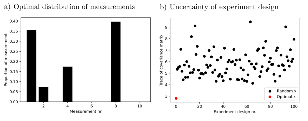
Finding a distribution \(x\) of measurements such that \(\operatorname{tr} ( \sum_{k=1}^{10} x_k a_ka_k^T)^{-1} \) is minimized is a semidefinite program that can be solved within 0.1 seconds on an office computer.

The result allows for some conclusions. For example, experiment No. 3 contributes little to the accuracy of the efficacy estimation, and experiment No. 2 is particularly informative. The above solution to the optimization problem achieves significantly better (= smaller) variances than other, randomly chosen experimental configurations.
Practical aspects
Optimal experimental design is particularly important when data collection involves significant effort and high costs, and the characteristics of the object under investigation are unclear. Special difficulties arise when correlations or causalities complicate the stochastic model \(l \approx A\theta\). The same applies to nonlinear relationships that prevent formulation as a well-defined semidefinite program.
However, if certain standard prerequisites are met, then optimal experimental design is routinely possible even with hundreds of measurement decisions to be made, and the interpretation of the guaranteed quality criteria is relatively straightforward.
Code & Sources
Example code: OD_experiment_design_1.py, OD_experiment_design_2 in our tutorialfolder
[1] Wolkowicz, H., Saigal, R., & Vandenberghe, L. (2012). Handbook of Semidefinite Programming: Theory, Algorithms, and Applications. Berlin Heidelberg: Springer Science & Business Media.
[2] Fletcher, R. (1981) A nonlinear Programming Problem in Statistics (Educational Testing). SIAM Journal on Scientific and Statistical Computing, 2(3), 257–267.
[3] Grafarend, Erik W., Sansò, F. (2012). Optimization and Design of Geodetic Networks. Berlin Heidelberg: Springer Science & Business Media.
[4] Ash, Robert B. (2011). Statistical Inference: A Concise Course. New York: Courier Corporation.
[5] Boyd, S., & Vandenberghe, L. (2004). Convex Optimization. Cambridge: Cambridge University Press.
[6] O’donoghue, B., Chu, E., Parikh, N., & Boyd, S. (2016). Conic Optimization via Operator Splitting and Homogeneous Self-Dual Embedding. Journal of Optimization Theory and Applications, 169(3), 1042–1068.
