Optimal design: Scheduling
Definition

In the design of schedules (= scheduling), the goal is to time a set of interdependent tasks in such a way that the total effort required to complete all tasks is minimized. The tasks in question can be industrial production processes, staff deployments, or simple room allocations.
Illustrations and quality criteria for schedules have been known since the early 20th century, and the Gantt charts developed during that period are still in use today. These charts allow existing schedules to be visualized in the form of bar diagrams, simplifying the communication of the plan contents and facilitating troubleshooting.
The design of schedules is carried out either manually according to heuristic rules or through optimization algorithms. The following example illustrates both approaches.
Example: Problem statement
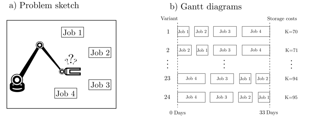
A machine has to perform 4 jobs \(J_1, …, J_4\). These jobs consume resource amounts \(r_1, …, r_4\) and require processing times \(p_1, …, p_4\).
| \(p_1\) | \(p_2\) | \(p_3\) | \(p_4\) | in days | \(r_1\) | \(r_2\) | \(r_3\) | \(r_4\) | in tons | |
|---|---|---|---|---|---|---|---|---|---|---|
| 5 | 6 | 10 | 12 | 1 | 1 | 1 | 1 |
The cost of storing the resources is directly proportional to the amount of resources stored and the storage time and should be minimized. The problem is small and simple to analyze and solve. For this purpose, all potentially possible Gantt diagrams are plotted.

Example: Cost minimization
The costs \(K\) are calculated as the sum of the resources to be stored and the storage durations according to the equation
$$\begin{align} K & = r_1(\text{Storage duration of resources for Job1})+ r_2(\text{Storage duration of resources for Job2})+… \\ & =\sum_{j=1}^4 r_jC_j \end{align}$$
where \(C_j\) is the completion time of Job \(j\). After comparing all variants, the best schedule turns out to be
$$\text{Job}_1 \rightarrow \text{Job}_2 \rightarrow \text{Job}_3 \rightarrow \text{Job}_4 \text{ with } K=r_1 5+r_2 11+ r_3 21+r_4 33=70.$$
It can even generally be shown [1, p. 131] that for the above system, an arrangement according to ascending processing times is optimal. If the resource quantities \(r_1, …, r_n\) are not all equal, then the WSPT rule (weighted shortest processing time first) applies: the ascending arrangement according to the quotients \(r_jp_j^{-1}\) is the optimal sequence and solves the optimization problem
$$\min_{\text{Schedule}} \sum_{j=1}^n r_jC_j.$$
Generalizations
If there are multiple different resources, processing machines, and constraints present, or if a different quality criterion is to be optimized, then there likely exist no optimal schedules that can be manually constructed following simple rules.
Instead, optimization algorithms must be employed. Often, these are mixed-integer optimization problems, which are computationally challenging to solve. A storage cost-minimizing schedule for \(n\) jobs on \(m\) machines can be formulated as the optimization problem [1, p. 134]
$$\begin{align} \min ~~~& \sum_{i=1}^m \sum_{j=1}^n \sum_{k=1}^nR_{ijk} p_{ij} x_{ikj} && \\ \text{s.t.} ~~~& \sum_{i=1}^m \sum_{k=1}^n x_{ikj}=1 &&j=1, …, n \\ & \sum_{j=1}^m x_{ikj} \le 1 && i=1, …,m ~ k=1, …, n \\ & x_{ikj}\in \{0,1\} && i=1, …, m ~ k=1, …, n ~ j=1, …, n \end{align}$$
Here, \(p_{ij}\) is the processing duration of job \(j\) on machine \(i\), and \(x_{ikj}\) is a binary indicator variable signifying whether job \(j\) is executed on machine \(i\) in the \(k\)-th last position. The constraints ensure that each job is assigned exactly once. The term \(R_{ijk}\) represents the resource quantities that need to be stored at the \(k\)-th last moment for processing on machine \(i\). These are the resource quantities for later projects on machine \(i\) that need to be stored over the duration \(p_{ij}\). Therefore, it follows:
$$R_{ijk} = \begin{cases} kr ~~~~~~~~~~~\text{ if } r_1=r_2= … = r_n =:r \\ \sum_{l\le k} x_{ikj}r_j \text{ otherwise }\end{cases} $$
In the case of unequal resource consumption, the optimization problem is nonlinear in the indicator variables \(x_{ikj}\) and can only be solved approximately, e.g., through relaxations based on semidefinite programming [2].
Example: m machines, n jobs
However, if all jobs use the same amount of resources, then with \(R_{ijk}=kr\) as the current storage quantity on machine \(i\), the optimization problem can be formulated as a linear program with the objective function
$$ \sum_{i=1}^m\sum_{j=1}^n \sum_{k=1}^nrkp_{ij}x_{ikj}$$
and the same constraints as above. This problem can be solved, for example, with the GLPK solver [3] for mixed-integer linear programming. As the following example shows, the optimal results cannot be achieved by intuitively guessing a job sequence or tabulating all potential solutions. It involves minimizing resource storage costs for 12 jobs on 3 machines. The processing durations \(p_{ij}\) are as follows:
| Machine\ Job | 1 | 2 | 3 | 4 | 5 | 6 | 7 | 8 | 9 | 10 | 11 | 12 |
|---|---|---|---|---|---|---|---|---|---|---|---|---|
| 1 | 1 | 1/2 | 2 | 1 | 1/2 | 1/4 | 3 | 2 | 1/8 | 1 | 2 | 1 |
| 2 | 1/2 | 2 | 1 | 1/2 | 1/4 | 3 | 2 | 1/8 | 1 | 2 | 1 | 1 |
| 3 | 2 | 1 | 1/2 | 1/4 | 3 | 2 | 1/8 | 1 | 2 | 1 | 1 | 1/2 |
The corresponding linear program is
$$\begin{align} \min ~~~ & q^T \operatorname{vec} (x) \\ \text{s.t.} ~~~ & x^TA=\vec{1} \\ & xG \le \vec{1} \\ & x_{ikj}\in \{0,1\} \end{align} $$
where \(q\in \mathbb{R}^{mn^2}, A=[1, …, 1]^T \in \mathbb{R}^{mn}, G=[1, …, 1]^T \in \mathbb{R}^n\). Here, \(\operatorname{vec}\) is the vectorization operator, which remodels matrices into vectors. The matrices and vectors are defined as
$$\begin{align} q & = \operatorname{vec}(Q) ~~~~(Q)_{ikj}=kp_{ij} \\ x & = \begin{bmatrix} x_{111} & \cdots & x_{11n} \\ \vdots & \ddots & \vdots \\ x_{311} & \cdots & x_{31n}\\ x_{121} & \cdots & x_{12n} \\ \vdots & \ddots & \vdots\\ x_{3n1} & \cdots & x_{3nn} \end{bmatrix} \in \mathbb{R}^{mn \times n}\end{align}$$
Example: Solution
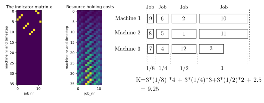
The result (GLPK, 60 ms) is given by the following matrix and associated Gantt-chart.

The objective function attains the value 9.25. Compare this to the following randomly selected schedule.

The costs associated to this schedule are
$$\begin{align} K =& p_{11}(4)+ p_{12}(3)+p_{13}(2)+p_{14}(1)\\ & +p_{25}(4)+p_{26}(3)+p_{27}(2)+p_{28}(1) \\ & + p_{39}(4)+p_{310}(3)+p_{311}(2)+p_{312}(1) \\& = 4(1+1/4+2)+3(1/2+3+1)+2(2+2+1)+1(1+1/8+1/2) \\ & = 38.125 \end{align} $$
These costs are more than 4 times as high as those of the optimal schedule.
Practical aspects
With 12 jobs, a naive approach to check all job arrangements would already be challenging. For just one of the machines, there would be \(12! \approx 500 000 000\) arrangements to explicitly list and evaluate regarding their constraints and resource consumption. With three machines, it surpasses \(10^{16}\), which exceeds the capabilities of normal office computers.
There are various other constraints and objective functions. Typical ones include [1, pp. 14–20]:
- Machine setups: Single machine, identical machines, machines with different work speeds, independent machines, flow jobs, job shops, etc.
- Constraints: Interruptibility of jobs, sequence conditions, setup times, waiting times, deadlines, job groups, machine restrictions, batch processing, etc..
Objective functions: Sum of completion times, keeping to processing ends and deadlines, sum of delays, etc.
For many of the above combinations, it’s not straightforward to formulate and solve them as mixed-integer programs. However, mathematical scheduling can tackle problems that manual planning cannot due to complexity reasons.
Code & Sources
Example code: OD_scheduling.py in our tutorialfolder
[1] Pinedo, Michael L. (2016). Scheduling: Theory, Algorithms, and Systems. Berlin, Heidelberg: Springer.
[2] Bansal, N., Srinivasan, A., & Svensson, O. (2016). Lift-and-round to improve weighted completion time on unrelated machines. Proceedings of the forty-eighth annual ACM symposium on Theory of Computing. Association for Computing Machinery, New York, NY, USA, 156–167.
[3] GNU Linear Programming Kit: https://www.gnu.org/software/glpk/
