Applications: Statistics and optimal estimation
Definition

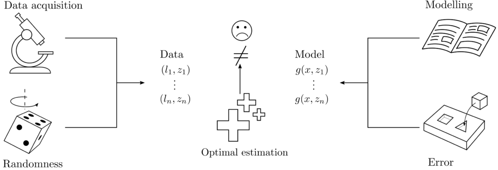
Mathematical statistics involves methods for collecting, analyzing, and evaluating data. The goal is to derive usable information in the form of statistical metrics and the optimal estimation of relationships fraught with uncertainty.
Optimality in estimating parameters, unknown functional relationships, uncertainties, etc., is achieved by maximizing probabilities conditioned on available data. Optimal estimation is necessary wherever real-world complexities impede the unambiguous solvability of a problem.
Example
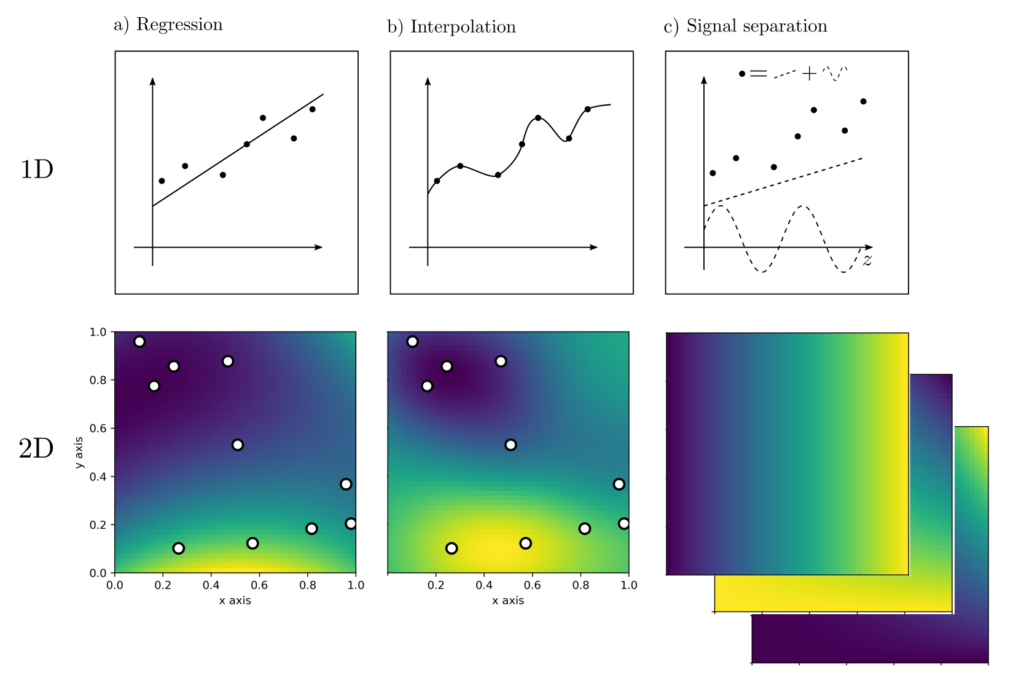
This is often the case when information is to be extracted from measurement data. Measurement data are subject to random and systematic fluctuations, stemming from imperfections in the measurement system and dynamic influences of the environment acting on the system. Data are typically contradictory and must be processed before they are useful. Based on a series of measured values at positions \(z_k, k=1, …, n\), various questions can be relevant:
- Regression. Find parameters of a model that best explain the observations.
- Interpolation. Estimate measurement values at positions where no measurements have taken place.
- Signal separation. Decompose the measured values into systematic and random components.
- Uncertainty estimation. Quantify the uncertainties in the information derived from data.

Explanation regression
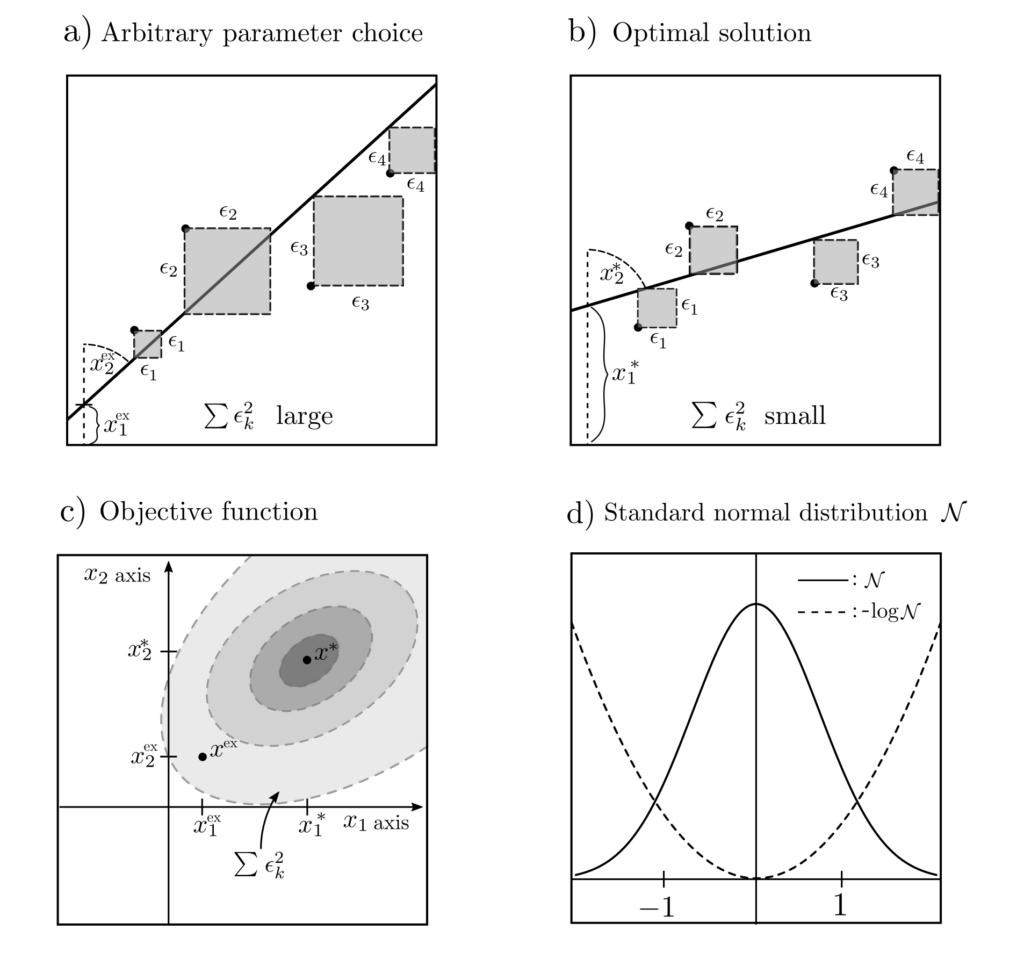
In the example illustrating regression, the values \(l_k, k=1, …, n\) have been observed at the positions \(z_k, k=1, …, n\). Now the parameters \(x\) are to be chosen such that predictions \(g(x,z_k)\) and observations \(l_k\) match as closely as possible. The predictive model in the depicted 1D case is the linear equation
$$ g(x,z)=x_1+x_2z$$
which predicts the observation \(g(x,z)\) at any position \(z\). More complex models are also possible. They can take the form \(g(x,z)=\sum_{k=1}^{m_1}x_kg_k(z_1, …, z_{m_2})\) with \(m_1\) parameters \(x=[x_1, …, x_{m_1}]\) and \(m_1\) different functions \(g_k(z_1, …, z_{m_2})\) depending on a \(m_2\)-dimensional position variable \(z=[z_1, …, z_{m_2}]\).
The requirement for a probability-maximizing choice of the parameter vector \(x\) can be formalized as the optimization problem
$$ \begin{align} \max_x ~~~& p(l_1, …, l_n, z_1, …, z_n | x_1, x_2) \end{align}$$
where the objective function \(p(l,z|x)\) indicates the probability of an observation \(l\) at the position \(z\) when the parameters are set to \(x\).
Least squares
Assuming \(l=x_1+x_2z+\epsilon\) with \(\epsilon\) being standard normally distributed noise, the probability reformulates as
$$ p(l_1, …, l_n, z_1, …, z_n|x_1,x_2) = \prod_{k=1}^n p(l_k,z_k|x_1,x_2)= c \exp\left(-\sum_{k=1}^n \frac{1}{2}[l_k-x_1-x_2z_k]^2\right).$$
The constant \(c\) is irrelevant for maximizing the probabilities \(p(l,z|x)\) or minimizing \(-\log p(l,z|x)\), and the following optimization problem results.
$$ \begin{align} \min_{x_1, x_2} ~~~& \sum_{k=1}^n \left[l_k-x_1-x_2z_k\right]^2 \\ =\min_{x_1, x_2} ~~~& \|l‑Ax\|_2^2 \\ ~~~& \|l‑Ax\|_2^2=(l‑Ax)^T(l‑Ax) \\ ~~~& A=\begin{bmatrix} 1 & z_1 \\ \vdots & \vdots \\ 1 & z_n \end{bmatrix}^T ~~~ l = \begin{bmatrix}l_1 \\ \vdots \\ l_n\end{bmatrix} \end{align}$$
This is a simple quadratic program without constraints that can actually be solved by hand for the optimal \(x^*=(A^TA)^{-1}A^Tl\). This formulation is known as the least squares problem, since it minimizes the squares of the discrepancies between measured and predicted values.

Other tasks
Interpolation, signal separation, and uncertainty estimation can also be formulated as optimization problems.
Interpolation:
Minimize \(\|x\|_{\mathcal{H}_2}^2\) subject to \(Ax = l\), where \(x \in \mathcal{H}_2\).
Signal Separation:
Minimize \(\|Ax‑l\|_{\mathcal{H}_1}^2 + \|x\|_{\mathcal{H}_2}^2\) subject to \(x \in \mathcal{H}_2\).
Uncertainty Estimation:
Minimize \(\langle \Sigma, P \rangle_F + 2q^T\mu + r\) subject to \(\begin{bmatrix} P & q \\ q^T & r \end{bmatrix} \succeq \tau_i \begin{bmatrix} 0 & a_i/2 \\ a_i^T/2 & ‑b_i \end{bmatrix}\) and \(\begin{bmatrix} P & q \\ q^T & r \end{bmatrix} \succeq 0\).
More details on the precise meaning of the quadratic and semidefinite programs can be found on the subsequent pages.
Solution procedures
When the number of data points to be integrated into the model is not overwhelmingly large, optimization problems can be solved using publicly available open-source solvers. This is typically the case. However, when dealing with several hundred thousand or millions of data points, numerical complications may arise, which can be mitigated by intelligently leveraging underlying problem structures.
To avoid processing huge correlation matrices with \(n^2\) entries (where \(n\) is the number of data points), tensor decomposition and numerical inversion are used. Stochastic gradient descent, well-known from machine learning, also bypasses the large matrices encountered in holistic data evaluation by sequentially processing the data. These strategies are rarely necessary when dealing with time series, audio data, or spot measurements but are essential when processing automatically generated multidimensional data from cameras or radar instruments.
Applications
Every practical problem involves unknown quantities and relationships, which is why methods of statistics and optimal estimation are now encountered everywhere. Applications include the optimal estimation of travel times, house prices, ore grades, material properties, building deformations, flight trajectories, and the chemical compositions of distant planets. Furthermore, they include the analysis of winning probabilities in sports or the failure probability of components, the decomposition of measurement data into signal and noise, the identification of objects in images, and model building for the spread of diseases or political opinions. More applications can be found in this list.
Optimal estimation is the response to the ubiquitous presence of data and model uncertainties.

Practical aspects
The main challenge in setting up optimal estimation problems with real-world backgrounds lies in how random elements in the data and models can be represented. At a minimum, this requires recourse to probability theory, and stochastic modeling of random effects requires experience with probability distributions tailored to various situations, more on this here.
In many cases, the optimal estimation of parameters or function values can be reduced to a least-squares problem and even solved manually. However, when non-normally distributed variables are involved, the probabilities to be maximized can quickly take on a complex form, and dedicated optimization algorithms are required.
Code & Sources
Example code: OE_interpolation_regression.py , OE_simulation_support_funs.py in our tutorialfolder
