Estimation correlation structures

Optimal estimation: Estimation of correlation structures

Definition

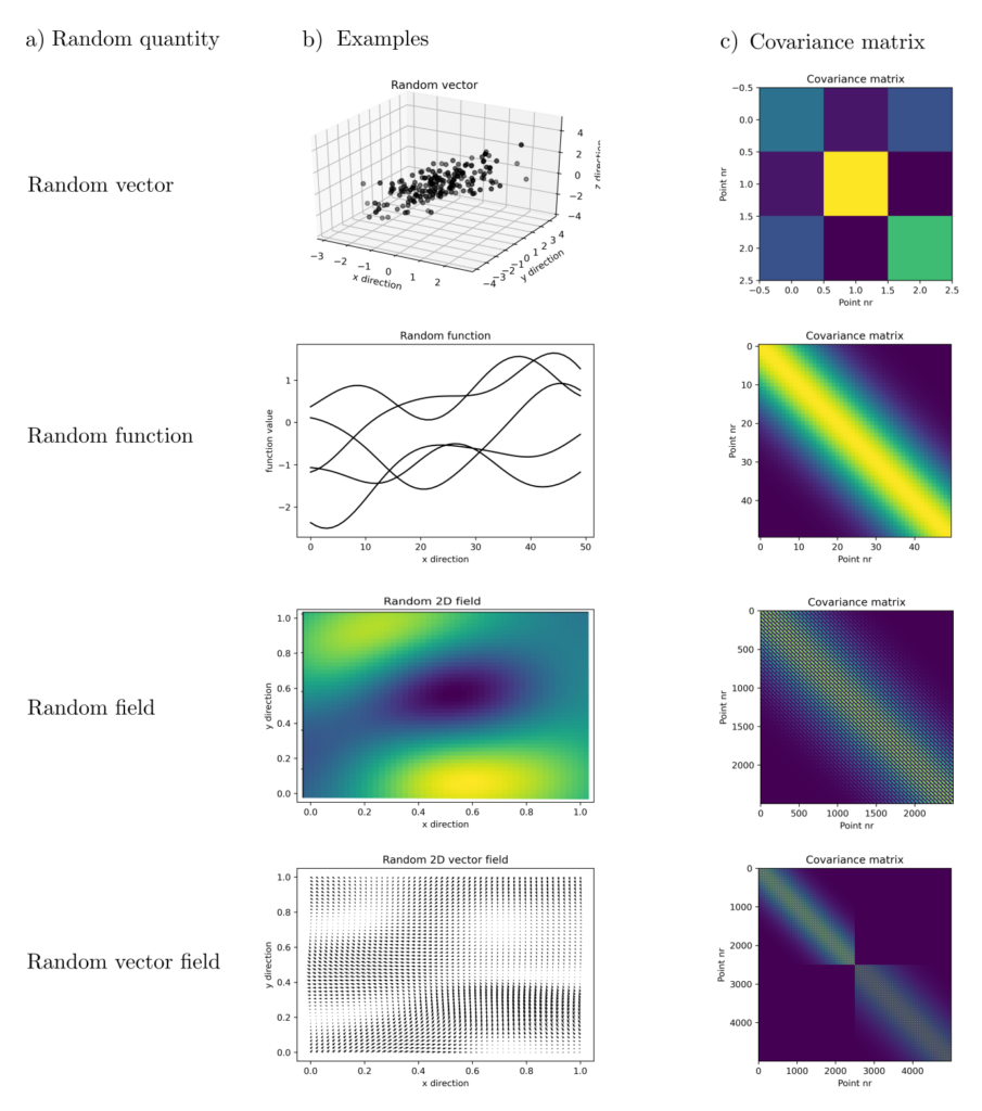
Correlation structures describe the relationships between function values $f(z_1), … , f(z_n)$ without prescribing an explicit functional form of $f$. The most common are the so-called covariance matrices $C$. They fully encode the correlations among all function values.

Each entry of $C$ represents the covariance between two random variables $f_i, f_j$.

$$ C= \begin{bmatrix} c_{11} & \cdots & c_{1n} \\ \vdots & \ddots & \vdots \\ c_{n1} & \cdots & c_{nn}\end{bmatrix} ~~~~~~ c_{ij}=E[f_if_j]-E[f_i]E[f_j]$$

Here, $E[f_i]$ is the expected value of the random variable $f_i$. The equation implies that $C$ is a symmetric matrix with dimensions $n \times n$, where $n$ is the number of all random variables.

Problem statement

If covariance matrices are fully known, they are an essential part of the equations for optimal estimation. Often, however, this is not the case, and functions $K(z_1, z_2) = E[f_{z_1}f_{z_2}] — E[f_{z_1}]E[f_{z_2}]$ must be estimated from sporadically available data $f_1, …, f_n$. These covariance functions $K(z_1, z_2) : Z \times Z \rightarrow \mathbb{R}$ are then used to generate the covariance matrices of all sizes needed for optimal estimation.

Deriving the covariance function $K$ from data $f_1, …, f_n$ presents a challenge. Since covariance matrices must be positive semidefinite, $K$ must satisfy

$$ C \succeq 0 ~~~~~~ C_{ij} = K(z_i, z_j) $$

regardless of the specific sequence of evaluation points $\{z_i\}_{i=1}^n \subset Z$ [1, p. 11]. Such $K(\cdot, \cdot)$ are called positive definite kernels. Deriving $K(\cdot, \cdot)$ from data requires solving a statistical inference problem with constraints concerning the spectrum of matrices constructible from $K(\cdot, \cdot)$. This is not a straightforward problem.

Relevance

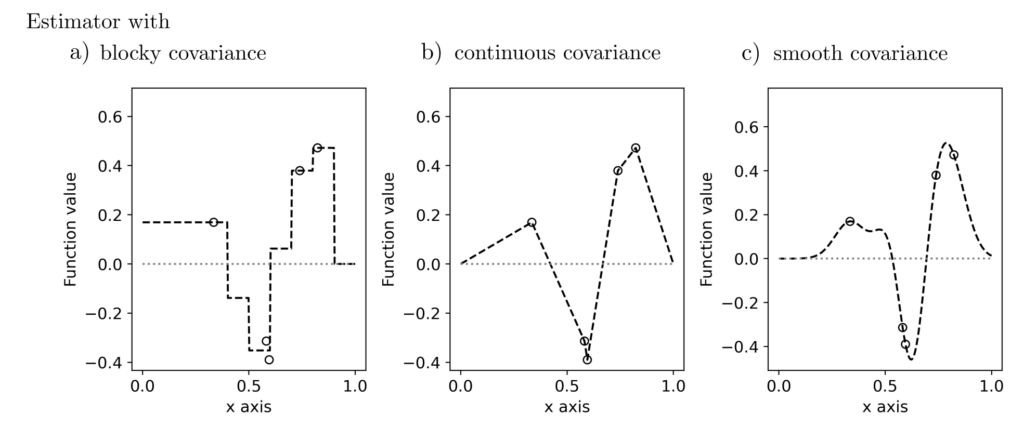
Despite its complexity, it remains a crucial problem and an essential prerequisite for truly reliable optimal estimation, as demonstrated, for example, in the equations for solving the interpolation problem. The optimal estimator $f(\cdot)$ based on observations $l = [f(z_1), …, f(z_n)]^T$ is:

$$ \begin{align}
f(z) & = \operatorname{argmin} \|f\|_{\mathcal{H}_K}^2 \\
& \text{s.t.} f(z_j) = l_j, \quad j = 1, …, n \\
& = \begin{bmatrix} K(z, z_1) & \cdots & K(z, z_n) \end{bmatrix} \begin{bmatrix} K(z_1, z_1) & \cdots & K(z_1, z_n) \\ \vdots & \ddots & \vdots \\ K(z_n, z_1) & \cdots & K(z_n, z_n) \end{bmatrix}^{-1} \begin{bmatrix} l_1 \\ \vdots \\ l_n \end{bmatrix} \\
& = \sum_{j=1}^n \alpha_j K(z, z_j)
\end{align}$$

Thus, it depends only on the data and the covariance function. For stochastic processes, knowledge of the covariance function is often equivalent to knowing the entire probability distribution and thus is a central component of the estimation equations. Consequently, the impact of the covariance function on the optimal estimator is significant.

Functional model for covariance functions

Similar to the representation of positive semidefinite matrices $C$ as the product $B^TB$ of matrices $B$, a covariance function can always be written as $\int_Z B(z_1,z)B(z,z_2)dz$. Under some assumptions [2, pp. 158–163], this implies a decomposability of $K(z_1,z_2)$ into

$$ K(z_1,z_2)=\sum_{i=1}^{\infty}\sum_{j=1}^{\infty} \gamma_{ij}\varphi_i(z_1)\varphi_j(z_2) $$

where $\varphi_i(z), i=1, … $ form an orthonormal basis of functions on $Z$ and $\gamma \succeq 0$ is a positive semidefinite matrix that approximately follows a Wishart distribution. This model is very flexible and can generate a variety of correlation structures.

Inference equations

Assuming $K(z_1,z_2)$ is a square $B^TB = \int_Z B(z_1,z)B(z,z_2)dz$ of normally distributed random functions $B$, then $\gamma$ is approximately Wishart distributed. With $p(l|\gamma)$ being the conditional probability of observations $l$ given the covariance function dependent on $\gamma$ and $p(\gamma)$ the probability of $\gamma$, according to Bayes’ theorem,

$$p(\gamma|l) = c p(l|\gamma)p(\gamma) ~~~~~~ c \text{ a constant}.$$

Here, $p(\gamma|l)$ is the conditional probability of $\gamma$ when $l$ has been observed. Maximizing the probability is equivalent to minimizing $-\log p(\gamma|l)=-\log p(l|\gamma)-\log p(\gamma)$.

The optimization problem is formulated as

$$ \begin{align} \min_{\gamma} ~~~& \log \det C_{\gamma} + \operatorname{tr} (SC_{\gamma}^+)+ r\left[ — \log \det \gamma + \operatorname{tr}(\Lambda^+\gamma)\right] \\ \text{s.t.}
~~~& A \gamma =b \\ ~~~& \gamma \succeq 0 \end{align}$$

where $S$ is the empirical covariance matrix of the data $l$, $C_{\gamma}$ is the covariance matrix reconstructed using $\gamma$, $C_{\gamma}^+$ its pseudoinverse, and $\Lambda$ a matrix encoding a‑priori assumptions about $\gamma$. The regularization constant $r$ balances prior knowledge and data, and $A \gamma = b$ are linear conditions for $\gamma$ representing definite knowledge about underlying correlations. With information about first and second derivatives of the objective function, the following numerical scheme emerges [2, p. 194]

$$ \begin{align} \gamma &= \gamma +\Delta \gamma ‑A^T(A\gamma A^T)^+A\Delta \gamma \\ \Delta \gamma & = \frac{1}{1+r} \left[ (r‑1)\gamma +S_{\psi} — r\gamma \Lambda^+\gamma\right] \end{align}$$

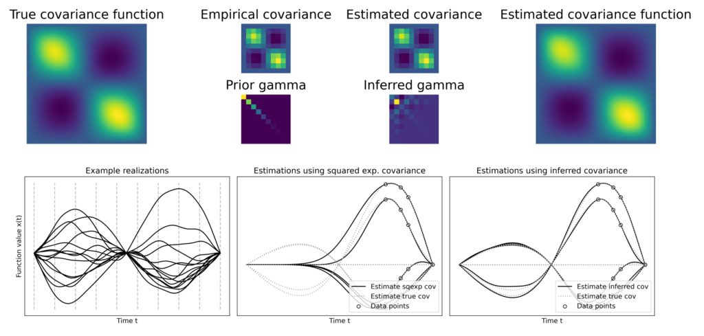
where $S_{\psi}$ is a transformed version of the empirical covariance matrix. When iterations over $\gamma$ are numerically stabilized and carried out to convergence, the result is a covariance function $ K(z_1,z_2)$ constructed using $\gamma$. This predicts for all possible positions $z_1, z_2$ the associated correlations ensuring they are maximally consistent with the point observations $l$ and the prior assumptions.

Results

The optimal estimation of correlation structures using the above method is more flexible than the classic approach based on the subjective choice of parametric families of covariance functions. A variety of real-world processes cannot be represented by simple functions in terms of their correlation structure.

The stochastic modeling of such processes benefits from the flexibility of the above method. This becomes particularly evident when covariance functions derived from various methods are used within the framework of optimal function estimation.

Figure 4: The underlying true covariance function is typically unknown. Only individual measurements are accessible, along with a conjecture about, for example, the smoothness properties of the covariance function. When data and prior knowledge are combined, a covariance function is created that closely resembles the true one. Note that this covariance function leads to significantly better interpolations than a generic covariance function.

Extensions

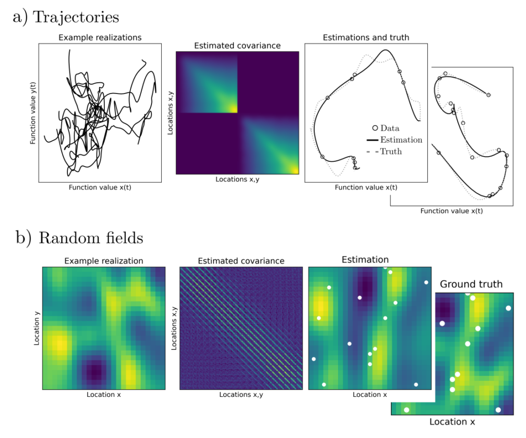
The estimation procedure can be extended to situations where both means and covariances are unknown and observations $l$ fall into $m$ different groups $(l^1_1, …, l^1_{n_1}, … l^m_1, …, l^m_{n_m})$ with varying data collection methodologies. The corresponding optimization problem is:

$$ \begin{align} \min_{\beta, \gamma} ~~~& \sum_{i=1}^m \log \det \eta_i + \operatorname{tr} (S_{\phi}^i\eta_i^+)+ r\left[ — \log \det \gamma + \operatorname{tr}(\Lambda^+\gamma)\right] \\ \text{s.t.} ~~~& A \gamma =b \\ &F_i\gamma -\eta_i= 0 ~~~~ i=1, …, m \\ ~~~& \gamma \succeq 0 \\ & \eta_i \succeq 0 ~~~~ i=1, …, m \end{align}$$

where $\eta_i, i=1, …, m$ are covariance matrices linked to $\gamma$ through $F_i\gamma-\eta_i=0$ and $S_{\phi}^i$ are transformed empirical covariance matrices. The optimization can be performed using a projected Newton method, see here (Github Link). The extension to multiple dimensions is straightforward.

Practical aspects

The estimation of correlation structures is very important for generating meaningful stochastic models and is therefore a frequent topic of discussion in spatial statistics, the analysis of physical processes, the use of regression models, and in machine learning.

If sufficient data is available, a stochastic model created manually based on assumptions can be refined, which positively affects the quality of the statements derived using the model.

Code & Sources

Example code: OE_KI.py , OE_KI_support_funs.py , OE_KI_covariance_impact_1.py, OE_KI_covariance_impact_2.py , OE_KI_interpolate_brownian_bridge.py , OE_KI_interpolate_field.py , OE_KI_interpolate_function.py , OE_KI_interpolate_trajectgory.py in our tutorialfolder.

[1] Berlinet, A., & Thomas-Agnan, C. (2011). Reproducing Kernel Hilbert Spaces in Probability and Statistics: . Berlin Heidelberg: Springer Science & Business Media.

[2] Butt, J. A. (2019). An RKHS approach to modelling and inference for spatiotemporal geodetic data with applications to terrestrial radar interferometry. Dissertation ETH Zürich, Zürich.