Methods: Mixed integer Programming
Definition

As soon as an optimization problem includes constraints concerning the integrality of variables, it is referred to as an Integer Program. The integrality requirement for a variable \(x_1\) is expressed as \(x_1 \in \mathbb{Z}\), where \(\mathbb{Z}\) represents the set of all integers.
When additional constraints are involved, including integrality constraints on some of the variables, the problem is referred to as a Mixed Integer Program (MIP). Depending on the form of the objective function \(f\) and the feasible set \(D\) in the optimization problem
$$ \begin{align} \min_x ~~~& f(x) \\ \text{s.t.}
~~~&x \in D \\ ~~~& x_1, …, x_m\in \mathbb{Z} \end{align}$$
it is classified as MILP (Mixed Integer Linear Program), MIQP (Mixed Integer Quadratic Program), MISDP (Mixed Integer Semidefinite Program), etc. Classic optimization problems can be enhanced with integrality constraints to make them more expressive.
Example 1
Consider \(x_1, x_2\) as the quantities of two products with manufacturing costs of \(c_1\) and \(c_2\) respectively. The constraints that their sum should cover a demand of 2 and that \(x_1, x_2\) can only be produced in discrete quantities translate into the optimization problem:
$$ \begin{align} \min_x ~~~& c_1x_1+c_2x_2 \\ \text{s.t.}
~~~&x_1 \ge 0 ~~~ x_2 \ge 0 \\ ~~~& x_1+x_2=2\\~~~& x_1, x_2\in \mathbb{Z} \end{align}$$
where \(x\) are the optimization variables. This variation of the archetypal production planning example is nearly trivial: The feasible set consists of the three elements \([0,2], [1,1], [2,0]\) and can be easily examined for its maximum. In this case, the inclusion of integrality has made the optimization problem simpler. However, this is not always the case.
Example 2
Another example shows that integrality is an unexpectedly flexible constraint. Consider the situation as in example 1; however, without the conditions \(x_1\in \mathbb{Z}, x_2\in \mathbb{Z}\). Instead, at least one of the contractual conditions \(x_1 \le 1.5\) or \(x_2\ge 1.5\) must be ensured. This can be formulated as a Mixed Integer Linear Program (MILP):
$$ \begin{align} \min_x ~~~& c_1x_1+c_2x_2 \\ \text{s.t.}
~~~&x_1 \ge 0 ~~~ x_2 \ge 0 \\ ~~~& x_1+x_2=2\\~~~& x_1 ‑M_1y_1 \le 1.5 ~~~~~~~~~~~~~~ M_1 \text{ upper limit for } x_1 \\ ~~~& ‑x_2 ‑M_2y_2 \le ‑1.5 ~~~~~~ M_2 \text{ upper limit for } ‑x_2 \\ ~~~& y_1+y_2=1 ~~~~ y_1,y_2\in \{0,1\} \end{align}$$
where \(x\) and \(y\) are the optimization variables. Here, \(y=[y_1,y_2]\) is either \([0,1]\) or \([1,0]\), indicating which of the two contractual conditions must be met.

Applications
The requirement for integrality is an unexpectedly flexible criterion. As shown in the example above, it can be used to formulate logically linked constraints [1, p. 6]. Using logical atoms such as AND, OR, and their combinations, entire decision trees can be embedded in optimization problems. Integer optimization thus also provides a basis for formulating solvability problems.
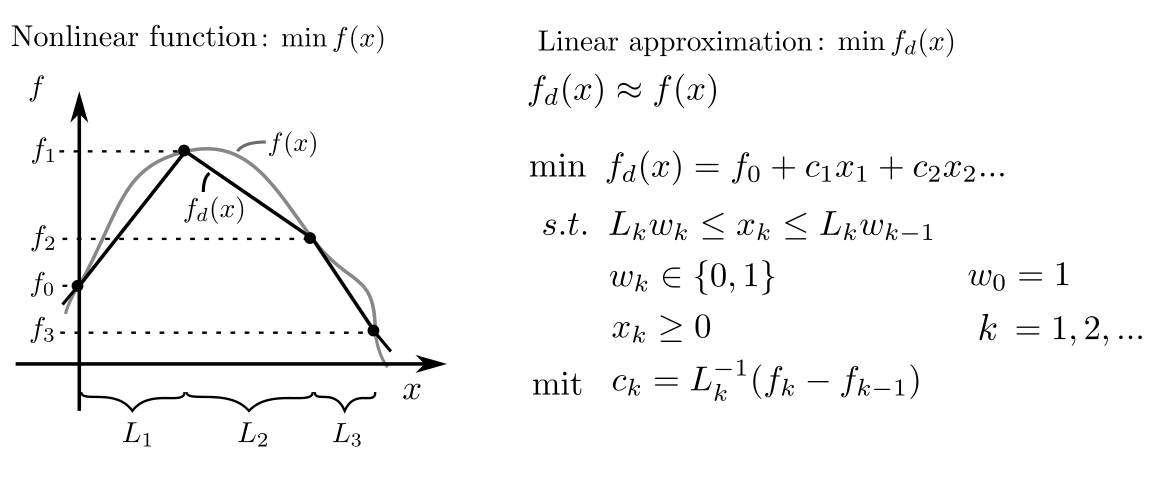
Furthermore, nonlinear terms in optimization problems can be represented as linear terms with integrality conditions [2, pp. 396–396].

It is evident that a formalism capable of representing and solving discrete, logical, and nonlinear problems has many applications. These are found, among other areas, in optimal control problems with discrete input options such as the regulation of stock-dependent fisheries, supermarket cold chains, aircraft control inputs, and collision avoidance. They also arise in optimal design problems with a discrete character, such as transportation network design, vehicle routing, goods flow control, factory layout, spatial arrangement of infrastructure, test sequencing and experimental design, storage space management, and logical feasibility problems. More information can be found here.
Solution procedure
Although integer optimization problems are generally very challenging, there are exact solution methods like the branch-and-cut algorithm that appear sufficiently powerful in practice. These methods are based on the construction of a tree structure of approximate LPs with an increasing number of linear constraints that collectively enforce the integrality conditions [2, pp. 396–413].
This tree structure can be efficiently searched using a combination of depth-first search and the pruning of tree components that are provably worse than previously evaluated solutions. An example of the implementation of such a solution algorithm is the GNU Linear Programming Kit with the GLPK_MI routine [3].
Practical aspects
Integer optimization problems are not always solvable in a reasonable time frame. They belong to the most expressive but also the most challenging problems known to mathematics and computer science [4]. From an empirical standpoint, however, they often work well enough for practical problems that do not exceed a few thousand integer variables. This is primarily a question of problem structure.
Some problem formulations are easy to interpret because they contain integer discrete objects as optimization variables. Often, however, nonlinear terms or logical constructs must be translated into constraints. This requires time, experience, and is not always feasible.
Code & Sources
Example code: Methods_milp.py in our tutorialfolder
[1] Appa, G. M., Pitsoulis, L., & Williams, H. P. (2006). Handbook on Modelling for Discrete Optimization. Berlin, Heidelberg: Springer.
[2] Vanderbei, Robert J. (2013). Linear Programming: Foundations and Extensions. USA: Springer US.
[3] GNU Linear Programming Kit: https://www.gnu.org/software/glpk/
[4] Padberg, M. (2005). Classical Cuts for Mixed-Integer Programming and Branch-and-Cut. Annals of Operations Research, 139, 321–352.
