Methods: Semidefinite programming
Definition

Under the term semidefinite programming (SDP), one understands optimization problems which have a linear objective function and whose constraints consist of linear equations and spectral inequalities which are less interpretable but more powerful than linear or quadratic inequalities.
Spectral inequalities quantify requirements on the spectrum (the eigenvalues) of matrices constructed from the optimization variables. Thus, the central optimization problems are:
$$ \begin{align} \min_x ~~~& \langle c, x\rangle \\ \text{s.t.}
~~~&Ax =b \\ ~~~& \sum_{k=1}^n x_k G_k \succeq 0 \end{align}$$
in the optimization variables \(x\) [1, p. 168]. Here, \(x, c, b\) are vectors, \(A, G_1, …, G_n, H\) are matrices and for a matrix \(F\), \(F\succeq 0\) means that the spectrum of \(F\) is positive. \(F \succeq 0\) is a global statement about certain combinations of all elements of \(F\) together and cannot be simplified to element-wise inequalities. The problem described in detail is as follows.
- Find the variables \(x_1, …, x_n\) such that \(\langle c,x\rangle = c_1x_1 +, … , +c_nx_n\) is minimized.
- The following should hold:
- \(a_{k1} x_1 + , …, + a_{kn}x_n =b_k ~~~~k=1, …, m_1\)
- \(x_1 G_1 + , …, + x_n G_n \succeq H\)
Like in LP, the problem consists of minimizing a sum \(\langle c,x\rangle\), \(m_1\) equations, and inequalities. Unlike LP, the inequalities pertain to the spectrum of the matrix \(x_1G_1 + , …, + x_nG_n‑H\), making them much more flexible but also harder to interpret. SDP is very general and includes LP, QP, QCQP, and SOCP [2, p. 3].
Example
Every example of LP, QP, QCQP, and SOCP is also an example of SDP. SDP is particularly suitable for optimization tasks concerning the eigenvalues of matrices, thus for example, minimizing uncertainty measures. Consider the matrix
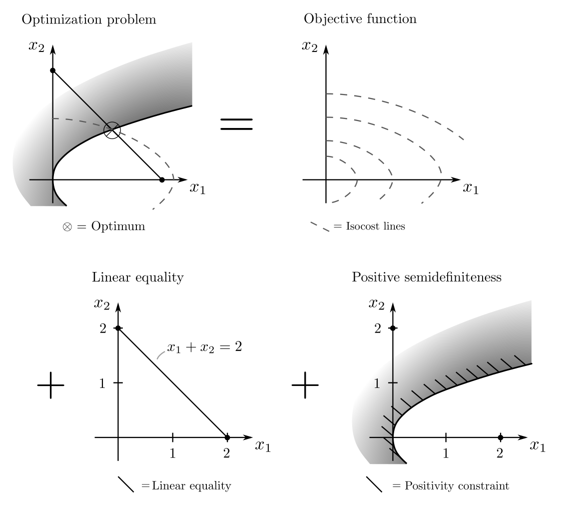
$$ \begin{align} F=\begin{bmatrix} x_1 & x_2 \\ x_2 &1 \end{bmatrix} \succeq 0 ~~~~~ x_1+x_2=2 \end{align}$$
which is the covariance matrix, a measure for the uncertainties and correlations in experiments. Here, \(x_1\) and \(x_2\) are decision variables concerning the choice of experiments. They should be chosen such that the largest eigenvalue of \(F\) — as an indicator of maximum uncertainty — is minimized. Through several transformations [1, p. 387], the problem can be written as the SDP
$$ \begin{align} \min_{x_1, …, x_n, t} ~~~& t \\ \text{s.t.}
~~~&x_1+x_2 =2 \\ ~~~& t \begin{bmatrix} 1 & 0 \\ 0 & 1\end{bmatrix} — \begin{bmatrix} x_1 & x_2 \\ x_2 & 1 \end{bmatrix} \succeq 0 ~~~~\begin{bmatrix} x_1 & x_2 \\ x_2 & 1 \end{bmatrix} \succeq 0 \end{align}$$
Using CVXPY [3] and the integrated SCS algorithm [4], the non-trivial solution \(x_1=1.6, x_2=0.4\) is obtained.

Applications
The applications of Semidefinite Programming (SDP) are enormously diverse and include all problems where the spectrum of matrices is relevant. These cover many probabilistic and physical issues; particularly in optimal control, system stabilization, control engineering, portfolio optimization, experimental design, statistical inequalities, robust approximation and decision making, structural engineering design, optimization under probabilistic constraints, and seeking approximation solutions for hard combinatorial problems such as Max Cut or the optimization of quadratic forms on graphs. Details can be found here.
The optimization variables \(x_1, …, x_n\) are often interpreted as parameters of covariance or energy matrices. Due to various tricks for formulating SDPs, they are often extremely difficult to understand. As an example, consider the embedding of Second Order Cone Programming (SOCP). These optimization problems of the form
$$ \begin{align} \min_x ~~~& \langle c, x\rangle \\ \text{s.t.}
~~~&Ax =b \\ ~~~& \|G_k x +h_k\|_2 \le \langle f_k,x\rangle + d_k ~~~ k=1, …, m_2 \end{align}$$
can be reformulated using the Schur complement as the SDP
$$ \begin{align} \min_x ~~~& \langle c, x\rangle \\ \text{s.t.}
~~~&Ax =b \\ ~~~& \begin{bmatrix} r_kI & q_k \\ q_k^T & r_k \end{bmatrix} \succeq 0 ~~~k=1, …, m_2 \end{align}$$
Here, \(I\) is the identity matrix, \(r_k=\langle f_k,x\rangle +d_k\), \(q_k=G_kx+h_k\), and the equivalence arises from \([A ~~b ; b^T~~ c] \succeq 0 \Leftrightarrow A\succeq 0 \wedge c- b^T Ab\succeq 0\).
Solution procedure
Semidefinite programs have been solvable with open-access software since the early 2000s, with theoretical algorithms existing since the 1980s [5]. As the illustrated example shows, optima do not necessarily occur on the boundary of the feasible set, which excludes methods like the Simplex method.
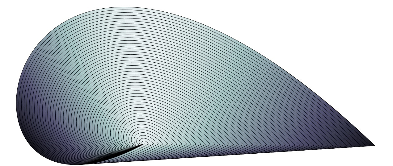
Instead, interior-point methods are used that replace conditions of the type \(X \succeq 0\) with barrier functions \(-\mu \log \det x\), which grow explosively at the edge of the feasible set. As \(\mu\) is successively reduced, the minimum of \(\langle c,x\rangle — \mu \log \det x\) approaches \(\min_x \langle c,x\rangle\) with \(x \succeq 0\) [6, p. 286]. The feasible sets are nonlinear and the path through the set is directed by local gradients, as shown in the figure.

Practical aspects
SDPs with tens of thousands of variables can be reliably solved today. The corresponding algorithms have been developed and implemented in the form of open-source software. SCS [4], SeDuMi [8], and SDPT3 [9] are publicly available—however, this software is numerically less stable than comparable solvers for LP or QP. Since the constraints in SDP can be considered as infinitely many linear inequalities, SDP is a very comprehensive problem class. However, modeling as a spectrally constrained optimization problem is a challenge.
Code & Sources
Example code: Methods_sdp.py in our tutorialfolder
[1] Boyd, S., & Vandenberghe, L. (2004). Convex Optimization. Cambridge: Cambridge University Press.
[2] De Klerk, E. (2006). Aspects of Semidefinite Programming: Interior Point Algorithms and Selected Applications. Berlin Heidelberg: Springer Science & Business Media.
[3] Diamond S., & Boyd S., (2016). CVXPY: A Python-embedded modeling language for convex optimization. Journal of Machine Learning Research, 17(83), 1–5.
[4] O’donoghue, B., Chu, E., Parikh, N., & Boyd, S. (2016). Conic Optimization via Operator Splitting and Homogeneous Self-Dual Embedding. Journal of Optimization Theory and Applications, 169(3), 1042–1068.
[5] Karmarkar, N. (1984). A new polynomial-time algorithm for linear programming. Combinatorica, 4, 373–395.
[6] Wolkowicz, H., Saigal, R., & Vandenberghe, L. (2012). Handbook of Semidefinite Programming: Theory, Algorithms, and Applications. Berlin Heidelberg: Springer Science & Business Media.
[7] Vinzant, C. (2014). What is … a spectrahedron? Notices of the American Mathematical Society, 61, 492–494.
[8] Sturm, J. F. (1999). Using SeDuMi 1.02, a MATLAB toolbox for optimization over symmetric cones. Optimization Methods and Software, 11(1–4), 625–653.
[9] Tütüncü, R. H., Toh, K. C., & Todd, M. J. (2003). Solving semidefinite-quadratic-linear programs using SDPT3, Mathematical Programming, 95, 189–217.
