Theory: Convexity
Definition

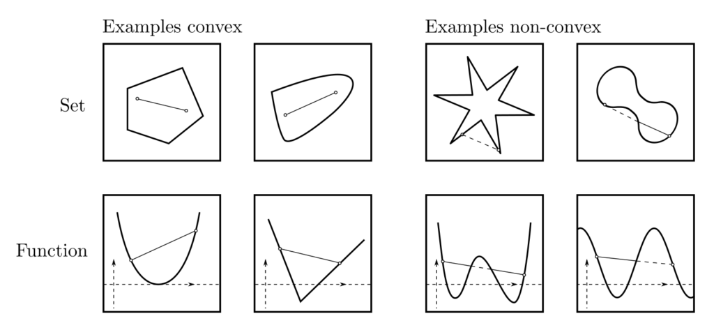
A set \(D\) is called convex if all its elements can be connected by straight lines that lie entirely within \(D\). Specifically, this means that for all \(x_1, x_2 \in D\) and \(y = \theta x_1 + (1-\theta)x_2\) with \(\theta \in [0,1]\), \(y\) is an element of \(D\).
Both \(x_1, x_2\) and \(y\) are vectors of arbitrary dimensions. Convex sets are simple objects in the sense that any point can be reached from any other point in a straightforward manner. A function \(f:D \rightarrow \mathbb{R}\) is called convex if \(D\) is convex and every linear approximation to \(f\) lies entirely above \(f\). Formally, this means that for all \(x_1, x_2 \in D\) and all \(\theta \in [0,1]\):
$$ \theta f(x_1) + (1-\theta)f(x_2) \ge f(\theta x_1 + (1-\theta) x_2) $$
The fact that the value of a convex \(f\) at any point \(x\) always lies below the average value of its neighbors implies the absence of hill-like shapes in the function landscape of \(f\) and a consistently upward (=positive) curvature. A comprehensive source on the convexity of sets and functions is [1, pp. 23–90].

Relevance
Convex sets and convex functions ensure unique and practically feasible minimizability. This is significant, as optimization problems are typically unsolvable [2, p.4]. As shown in the figure above, the presence of multiple minima implies that a function is not convex. Conversely, a convex \(f\) has only one local minimum.
Additionally, due to the convexity of \(f\), global properties can be inferred from local characteristics. Assuming \(f\) is differentiable, the following statements hold:
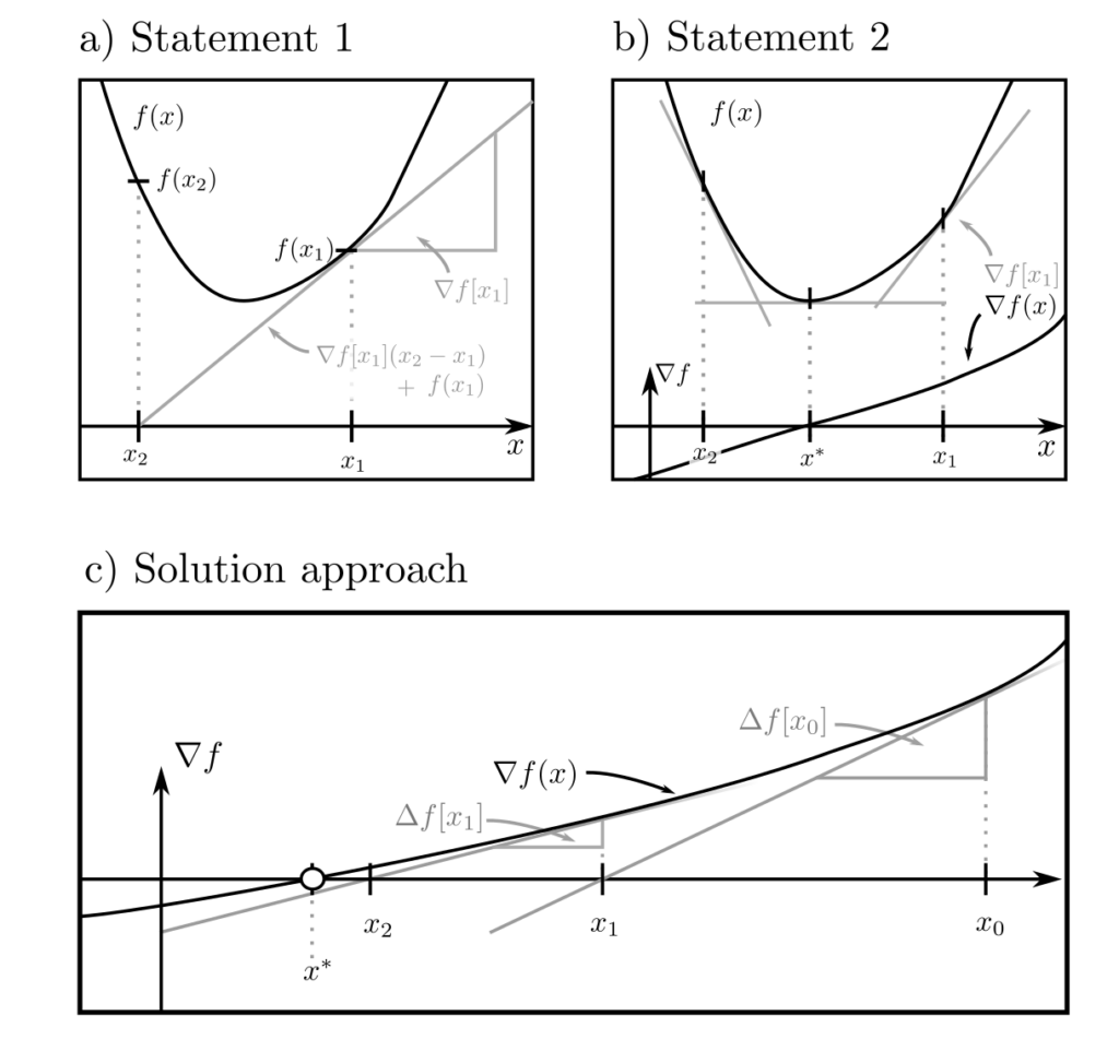
\(f(x_2) \ge f(x_1) + \nabla f(x_1)^T[x_2-x_1]\)
\(\Delta f(x)\succeq 0\)
for all \(x_1\) and \(x_2\), where \(\nabla f\) is the gradient (vector of first derivatives) and \( \Delta f\) is the Hessian matrix (matrix of second derivatives) of \(f\). A convex differentiable function is always non-negatively curved and is bounded below by its linear approximation. Consequently, the global minimum is at the point \(x^*\), where \(\nabla f(x)=0\). This follows from \(f(x_1)\ge f(x^*) + \underbrace{\nabla f(x^*)[x^*-x_2]}_{=0} \ge f(x^*)\).

Solution approach
The search for zeros of \(\nabla f\) leads directly to the method illustrated on the right in the above figure: Start at any point \(x_0\), use the value \(\nabla f(x_0)\) of the gradient and its rate of change \(\Delta f (x_0)\) to estimate the zero. With the estimator \(x_1\) for the zero, repeat the procedure until the actual zero \(x^*\) is found.
From \(\nabla f(x_0) + \Delta f[x_1 — x_0] \stackrel{!}{=} 0\), the sequence of estimators derived from \(x_0\) is given by $$ x_{k+1} = x_k — \Delta f^{-1}(x_k) \nabla f(x_k) ~~~~ k=0,1, … $$
This method is also known as the Newton method. Due to positive curvature, each point \(x_{k+1}\) has a lower function value \(f(x_{k+1})\) than its predecessor \(x_k\) and the method terminates at the optimum \(x^*\) [1, p. 484]. It can also be modified for optimization problems with constraints. More on this here.
Example
Many important functions are convex and can therefore be efficiently optimized. The examples in the following non-exclusive list are taken from [1, pp. 71–73].
| Name | Function | Domain | Application in modelling |
|---|---|---|---|
| Exponential function | \(e^{ax}\) | \(x\in \mathbb{R}, a \in \mathbb{R}\) | Growth processes and failure probabilities |
| Neg. logarithm | \(-\log x\) | \(x > 0\) | Probability distributions |
| Linear functional | \(c^T x\) | \(x\in \mathbb{R}^n, c \in \mathbb{R}^n\) | Combination of effects |
| Norm | \(\|x\|_p\) | \(x \in \mathbb{R}^n, p \ge 1\) | Discrepancies and distances |
| Neg. entropy | \(-\sum_{k=1}^n p(x_k)\log p(x_k) \) | \(p(x_k)> 0\) | Comparison probability distributions |
| Neg. geom. mean | \( — \left(\Pi_{k=1}^n x_k\right)^{1/n}\) | \( x\in \mathbb{R}^n, x_k >0\) | Growth processes and indicator functions |
| Maximum | \(\max (x_1, …, x_n)\) | \( x\in \mathbb{R}^n\) | Unproportional impacts |
| Softmax | \(\log \left( \sum_{k=1}^n e^{x_k}\right)\) | \( x\in \mathbb{R}^n\) | Machine learning |
| Neg. logdet | \(- \log \det X\) | \(X\) positiv definite | Covariance matrices and energies |
| Sum of eigenvalues | \( \sum_{k=1}^n \lambda_k(X)\) | \(X\) positiv semidefinite | Uncertainties and distributional properties |
| Matrix fractional | \(x^YP^{-1}x\) | \( x\in \mathbb{R}^n, P\) positiv semidefinite | Normal distributions and anisotropic distances |
Construction rules
The above examples can be combined to generate new, more expressive convex functions. Positively weighted linear combinations \(w_1f_1(x)+w_2f_2(x)\) of convex functions \(f_1(x), f_2(x)\) are convex; the same applies to the maximum \(\max( f_1(x),f_2(x))\) or the composition with a linear transformation to \(f_1(Ax+b)\). Modern modeling frameworks like CVXPY [3] leverage these relationships. Starting from demonstrably convex example functions and convexity-preserving composition rules, even seemingly complex functions can often be reduced to combinations of elementary convex functions and then solved [4].
Sources
[1] Boyd, S., & Vandenberghe, L. (2004). Convex Optimization. Cambridge: Cambridge University Press.
[2] Nesterov, Y. (2013). Introductory Lectures on Convex Optimization: A Basic Course. Berlin Heidelberg: Springer Science & Business Media.
[3] Diamond S., & Boyd S., (2016). CVXPY: A Python-embedded modeling language for convex optimization. Journal of Machine Learning Research, 17(83), 1–5.
