Theory: Stochasticity
Models and uncertainty
Uncertainty is an essential component of models that depict real-world phenomena. It can stem from various causes.
- The model involves phenomena of a random nature, such as nuclear decay, component failure, or stock prices.
- Dhe model includes deterministic but unknown quantities, such as the length of a not sufficiently accurately measured distance or the yet unpublished price of a product.
- The model is deliberately incomplete, and deviations between model behavior and reality are accounted for as uncertainty; for example, in problems of nonlinear continuum mechanics or feedback effects in complex systems.
In each of these cases, a part of the model is considered stochastic (=random). Regardless of whether the random element arises from the nature of the phenomenon or from ignorance of system parameters and relationships, it is described using the same formalisms of probability theory.
Random variables
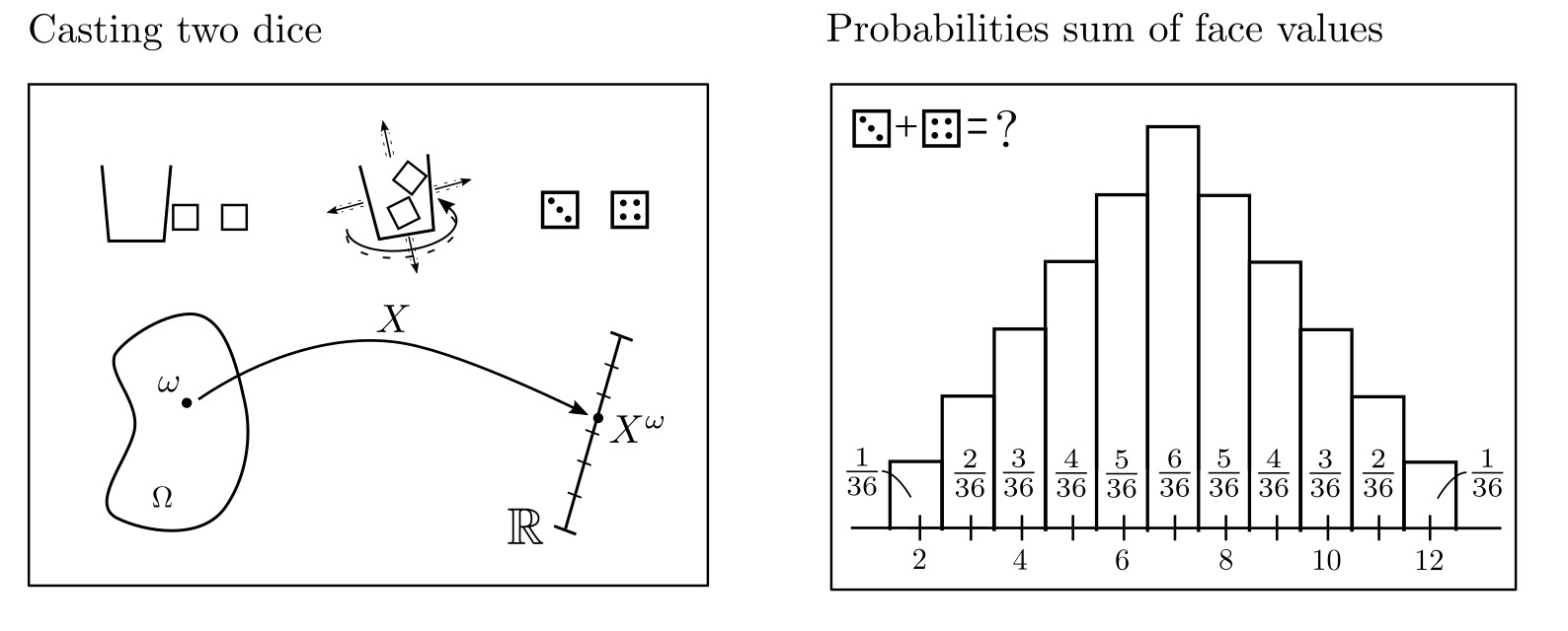
Random variables and their probability distributions play a central role. A random variable \(X^{\cdot}\) is a mapping $$X^{\cdot}:\Omega \ni \omega \mapsto X^{\omega}\in \mathbb{R}$$ which assigns a number to the result of an experiment [1, p. 46]. The experiment could be the roll of a die, the result being the upper face, and the random variable maps this result to the number of eyes. Before a die is actually rolled, the result of the experiment is not known, but it can be described in terms of the expected frequencies of possible eye counts. These relative frequencies are called probabilities; the assignment of probabilities to different numerical values is called a probability distribution.
Relevance
When a random variable \(X^{\cdot}\) appears in an optimization problem, all possible values of \(X^{\cdot}\) and their individual probabilities must be considered. This makes optimization problems harder to interpret. As the objective function is now random itself and characterized by a probability distribution, decisions must be made about the aspect of this distribution that is to be optimized.
For example, if the objective function is defined by costs \(c^Tx\) with the optimization variable \(x\in \mathbb{R}^n\) and random variables \([c_1^{\cdot}, …, c_n^{\cdot}]=c^T\), it may be sensible to minimize the expected value, the range of fluctuation, maximum values, or quantiles of the costs. Depending on the objective, this leads to linear programming (LP), semidefinite programming (SDP), or stochastic programs.
Typical probability distributions
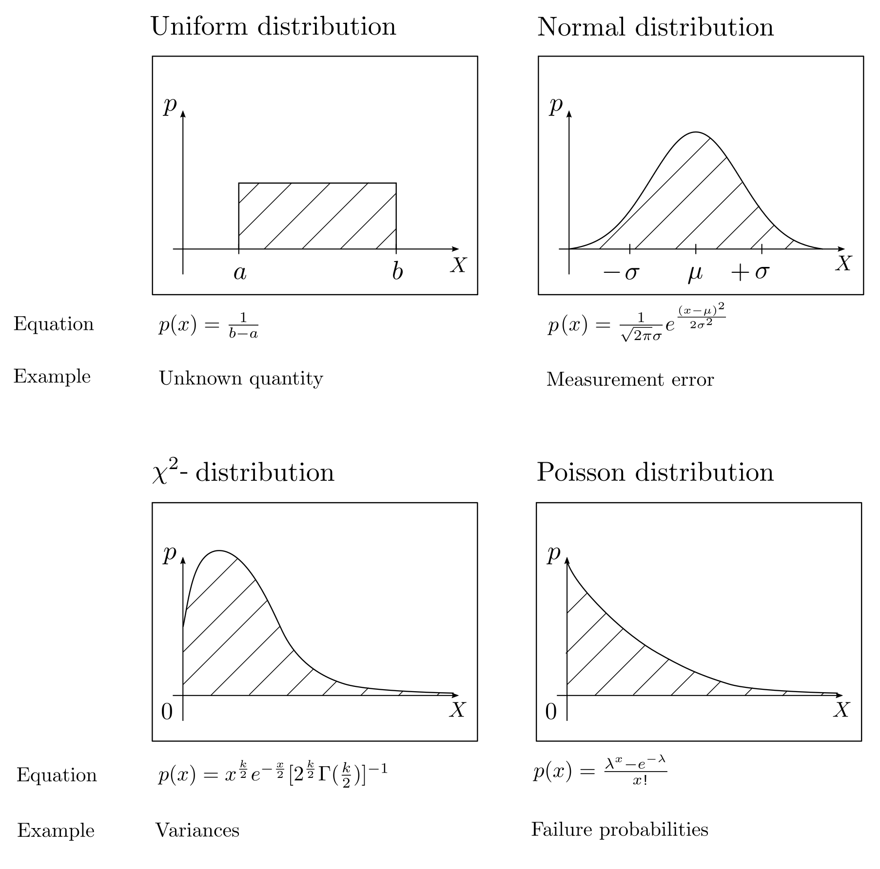
The most suitable probability distribution for modeling a random phenomenon depends on available background knowledge. Uniform distributions symbolize complete ignorance while normal distributions are good approximations for random effects composed of many independent minor errors. The \(\chi^2\)-distribution quantifies uncertainties related to lengths and distances, and the Poisson distribution can be used to describe failure probabilities. Various tailored probability distributions and their applications can be found in [2, pp. 828–828].
Stochastic processes
Multivariate probability distributions are especially relevant in practice. They quantify the probabilities of stochastic processes: collections of interrelated random variables associated with specific points in time, locations, or more generally any set of indices [1, p. 190]. Stochastic processes can be used to describe phenomena influenced by randomness in space or time, and even the simple multivariate normal distributions cover a wide range of potential behaviors to be modeled [3, pp. 79–94].
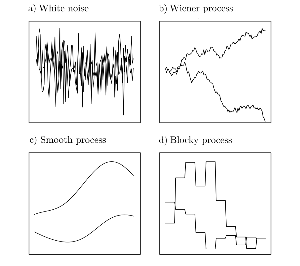
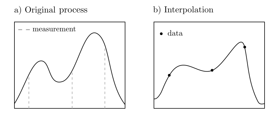
The illustrations demonstrate that even randomly generated functions can exhibit functional relationships. In principle, the assumption of stochasticity is seldom a hindrance, as stochastic models include deterministic models as a subset.
Exemplary application
Let \(X^{\cdot}_{\cdot}:T\times \Omega \ni (t,\omega)\mapsto X^{\omega}_{t} \in \mathbb{R}\) be a stochastic process; that is, a sequence of random variables indexed by the variable \(t\in T\). If the process has been observed only at certain times and is to be estimated for all other times based on these observations, this can be formulated as an optimization problem. Assuming a known probability distribution and hence known covariances, the best estimator \(\hat{X}_{t_0}\) for the value at \(t_0\) based on the observations \(X_{t_1}, …, X_{t_n}\) is given by
$$\hat{X}_{t_0} = \sum_{k=1}^n \lambda_k X_{t_k}.$$
Here, \([\lambda_1, …, \lambda_n]=\lambda\) is the solution to the quadratic program
$$\begin{align} \min_{\lambda} ~~~&\lambda^TC\lambda‑2\lambda^T c + \sigma_{00} \\
\text{s.t.} ~~~&\sum_{k=1}^n \lambda_k=1 \end{align}$$
where \(c\in \mathbb{R}^n\) with \(c_k=\text{Covariance}(X_{t_0},X_{t_j})\), \(C\in \mathbb{R}^{n\times n}\) with \(C_{kl}= \text{Covariance}(X_{t_k},X_{t_l})\), and \(\sigma_{00} = \text{Covariance}(X_{t_0},X_{t_0})\). This problem can be solved algorithmically or manually and leads to the method known as Kriging in geostatistics [4, pp. 163–164]. The value of the minimization problem is the variance of the estimation error.
Practical aspects
Uncertainties are part of all real-world phenomena and must be appropriately represented in optimization problems. This requires selecting probability distributions tailored to the phenomenon. Since it usually involves more than just one random variable, stochastic processes are used for modeling. These have high-dimensional probability distributions and must be incorporated into the optimization problem in a way that allows for meaningful solutions to be derived. This works well with multivariate normal distributions and uniformly distributed data but is challenging for less thoroughly studied probability distributions.
Code & Sources
Example code: Theory_stochastic_processes.py in our tutorialfolder
[1] Melsa, J. L., & Sage, A. P. (2013). An Introduction to Probability and Stochastic Processes. New York: Courier Corporation.
[2] Bronstein, I. N., Mühlig, H., Musiol, G. & Semendjajew, A. K. (2013). Taschenbuch der Mathematik. Haan-Gruiten: Verlag Europa-Lehrmittel
[3] Rasmussen, C. E., & Williams, C. K. (2005). Gaussian Processes for Machine Learning. Cambridge: MIT Press.
[4] Chilès, J. P., & Delfiner, P. (2009). Geostatistics: Modeling Spatial Uncertainty. New York: John Wiley & Sons.
